Scan, Attend and Read
Attention models for end-to-end handwritten paragraph recognition
Abstract
We present attention-based models for end-to-end handwriting recognition. Our systems do not require any segmentation of the input paragraph. The models are inspired by the differentiable attention models presented recently for speech recognition, image captioning or translation. The main difference is the implementation of covert and overt attention with a multi-dimensional LSTM network. Our principal contribution towards handwriting recognition lies in the automatic transcription without a prior segmentation into lines, which was critical in previous approaches. To the best of our knowledge this is the first successful attempt of end-to-end multi-line handwriting recognition. The experiments on paragraphs of Rimes and IAM databases yield results that are competitive with those of networks trained at line level, and constitute a significant step towards end-to-end transcription of full documents.
Acknowledgements. This work was carried out in the research team of A2iA. Please cite one of the following if you wish to refer to this work:
- Théodore Bluche (2016)
Joint Line Segmentation and Transcription for End-to-End Handwritten Paragraph Recognition.
In 30th Conference on Neural Information Processing Systems (NIPS 2016), to appear.
arXiv - Théodore Bluche, Jérôme Louradour, Ronaldo Messina (2016) Scan, Attend and Read: End-to-End Handwritten Paragraph Recognition with MDLSTM Attention. arXiv preprint arXiv:1604.03286.
Introduction
Several challenges are associated with offline handwriting recognition:
- the input is a variable-sized two dimensional image
- the output is a variable-sized sequence of character, with no direct relation to the input size
- the cursive nature of handwriting makes a prior segmentation into characters difficult
Early methods consisted in recognizing isolated characters, or in over-segmenting the image, and scoring groups of segments as characters (e.g. Bengio et al., 1995, Knerr et al., 1999). They were progressively replaced by the sliding window approach, in which features are extracted from vertical frames of the line image (Kaltenmeier, 1993). This approach formulates the problem as a sequence to sequence transduction. The two-dimensional nature of the image may be encoded with convolutional neural networks (Bluche et al., 2013) or by defining relevant features (e.g. Bianne et al. 2011).
The recent advances in deep learning and the new architectures allow to build models handling both the 2D aspect of the input and the sequential aspect of the prediction. In particular, Multi-Dimensional Long Short-Term Memory Recurrent Neural Networks (MDLSTM-RNNs, Graves et al., 2008), associated with the Connectionist Temporal Classification (CTC, Graves et al., 2006) objective function, yield low error rates and became the state-of-the-art model for handwriting recognition, winning most of the international evaluations in the field.
Up to now, current systems require segmented text lines, which are rarely readily available in real-world applications. A complete processing pipeline must therefore rely on automatic line segmentation algorithms in order to transcribe a document. Text recognition state-of-the-art moved from isolated character to isolated word recognition, then from isolated words to isolated lines recognition. This work follows the longstanding and successful trend of making less and less segmentation hypotheses for handwriting recognition.
We now suggest to go further and recognize full pages without explicit segmentation.
2014 and 2015 have seen a surge of interest in neural networks implementing a sort of attention mechanism, allowing the system to learn to focus on specific parts of its input in order to make predictions. Examples of successful applications are machine translation, speech recognition, or image/video description generation. I suggest reading this excellent article on RNNs with attention for a great tutorial on different mechanisms, applications, and references.
We propose to use attention mechanisms to get a model which can select a specific part of the image (i.e. a character or a line) in order to transcribe it. Interestingly, Fukushima wrote in 1993: "We believe that the use of selective attention is a correct approach for connected character recognition of cursive handwriting.". A few research papers were actually published in the nineties, which proposed an implementation of neural attention mechanisms stikingly similar to the models proposed recently (see for example Alpaydin, 1996; Mozer et al., 1998).
Handwriting Recognition with MDLSTM and CTC
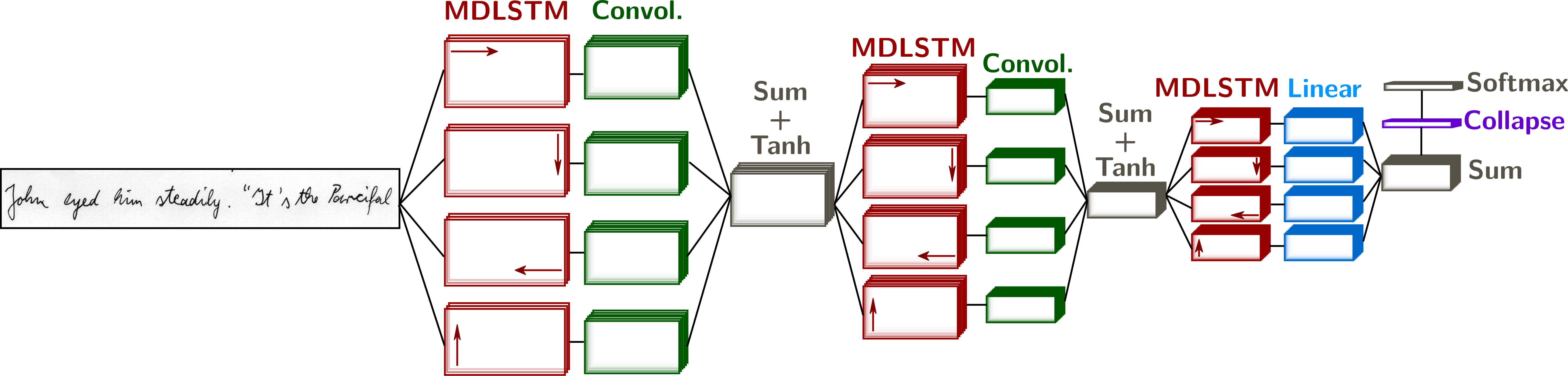
Multi-Dimensional Long Short-Term Memory recurrent neural networks (MDLSTM-RNNs) were introduced in (Graves et al., 2008) for unconstrained handwriting recognition. They generalize the LSTM architecture to multi-dimensional inputs. An overview of the architecture is shown in the figure above.
The image is presented to four MDLSTM layers, one layer for each scanning direction. The LSTM cell inner state and output are computed from the states and output of previous positions in the horizontal and vertical directions. The following equations illustrate the MDLSTM for the direction Left-to-Right, Top-to-Bottom.
The Input Gate controls whether the input of the cell is integrated in the cell state $$a^{i,j}_\iota = \sum_{i=1}^I w_{i\iota}x_i^{i,j} + \sum_{h=1}^H w_{h\iota} z_h^{i-1,j} + w_{h\iota'} z_h^{i,j-1}$$ $$z^{i,j}_\iota = f(a^{i,j}_\iota)$$ The Forget Gate controls whether the previous state is integrated in the cell state, or if it is forgotten. $$ a^{i,j}_{\phi_1} = \sum_{i=1}^I w_{i\phi}x_i^{i,j} + \sum_{h=1}^H w_{h\phi} z_h^{i-1,j} + w_{h\phi'} z_h^{i,j-1}$$ $$ z^{i,j}_{\phi_1} = f(a^{i,j}_{\phi_1})$$ $$ a^{i,j}_{\phi_2} = \sum_{i=1}^I w_{i\phi}x_i^{i,j} + \sum_{h=1}^H w_{h\phi} z_h^{i-1,j} + w_{h\phi'} z_h^{i,j-1}$$ $$ z^{i,j}_{\phi_2} = f(a^{i,j}_{\phi_2})$$ The Cell state is the sum of the previous state, scaled by the forget gate, and of the cell input, scaled by the input gate. $$ a^{i,j}_c = \sum_{i=1}^I w_{ic} x_i^{i,j} + \sum_{h=1}^H w_{hc} z_h^{i-1,j} + w_{hc'} z_h^{i,j-1}$$ $$ s^{i,j}_c = z^{i,j}_{\phi_1} s^{i-1,j}_c + z^{i,j}_{\phi_2} s^{i,j-1}_c + z^{i,j}_\iota g(a^{i,j}_c)$$ The Output Gate controls whether the LSTM unit emits the activation $h(s^{i,j}_c)$. $$ a^{i,j}_\omega = \sum_{i=1}^I w_{i\omega} x_i^{i,j} + \sum_{h=1}^H w_{h\omega} z_h^{i-1,j} + w_{h\omega'} z_h^{i,j-1}$$ $$ z^{i,j}_\omega = f(a^{i,j}_\omega)$$ The Cell output is computed by applying the activation function $h$ to the cell state, scaled by the output gate. $$ z^{i,j}_c = z^{i,j}_\omega h(s^{i,j}_c)$$
Each LSTM layer is followed by a convolutional layer, with a step size greater than one, subsampling the feature maps. As in usual convolutional architectures, the number of features computed by these layers increases as the size of the feature maps decreases. At the top of this network, there is one feature map for each label.
A collapse layer sums the features over the vertical axis, yielding a sequence of prediction vectors, effectively delaying the 2D to 1D transformation just before the character predictions, normalized with a softmax activation.
In order to transform the sequence of $T$ predictions into a sequence of $N \leq T$ labels, an additionnal non-character - or blank - label is introduced, and a simple mapping is defined in order to obtain the final transcription. The connectionist temporal classification objective (CTC, Graves et al., 2006), which considers all possible labellings of the sequence, is applied to train the network to recognize a line of text.
The Collapse Layer and its Proposed Replacements
The paradigm collapse/CTC already encodes the monotonicity of the prediction sequence, and allows to recognize characters from 2D images. The transformation from a 2D representation of the image (feature maps $\mathbf{e} = \{e_{ij}, i \in [1,H], j \in [1,W]\}$) is a simple sum across the vertical axis of the feature maps. Thus, the output $t$-th vector in the sequence is obtained through $$z_{t=j} = \sum_{i=1}^H e_{ij}$$ which means that
- all the feature vectors in the same column $j$ are given the same importance
- the same error is backpropagated in a given column $j$
- the output sequence will have length $W$, i.e. the width of the feature maps, so at most $W$ character can be recognized
- the ordering in the sequence will follow the same (spatial) ordering as the feature maps
The last point means that in general the image is "read" from left to right. Slight modifications may be brought to recognize languages with right-to-left reading order ($z_{t=j} = \sum_{i=1}^H e_{i,(W-j+1)}$) or top-to-bottom ($z_{t=i} = \sum_{j=1}^W e_{ij}$). Nevertheless, the reading order is not learnt but already implemented in the way the model is used with this formulation.
Point 2. (and 1., to some extent) also means that the intermediate features learnt by the network may not keep a two-dimensional interpretation. With this sum, we kind of force the network to predict a high score for one character on a whole column. This fact prevents from using intermediate representations for other text-related tasks that are not at the line level, and from recognizing several lines of text. When we look at the activations after the MDLSTM layers of a network trained on lines, applied on a whole paragraph, here is what we get:
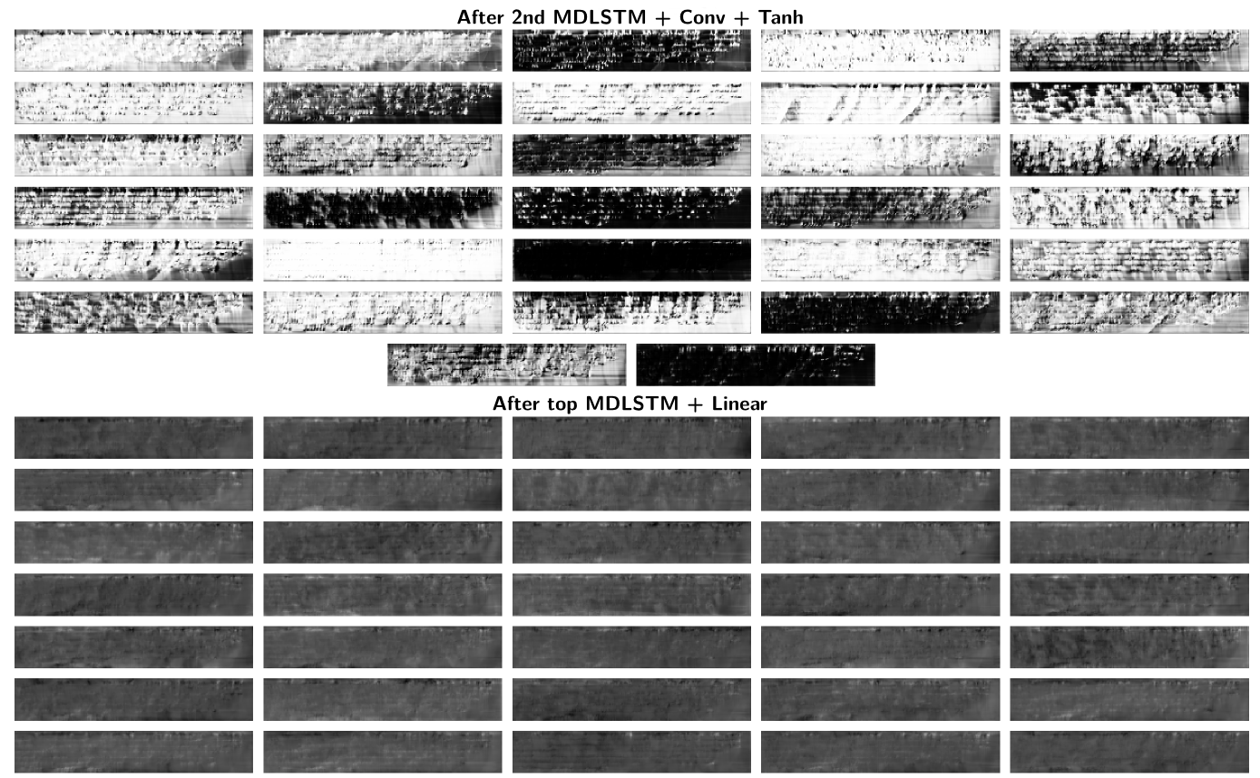
Although in some feature maps, we still see that the input image contains several lines of text, for most of them the network failed to generalize the feature extraction to multi-line images. (If you're not convinced, the activations of the same network, on the same image, trained with one of the presented attention methods is displayed later...).
In order to circumvent these limitations, and to enable the recognition of several lines, we proposed two modifications of the collapse layer, illustrated in the following figure:
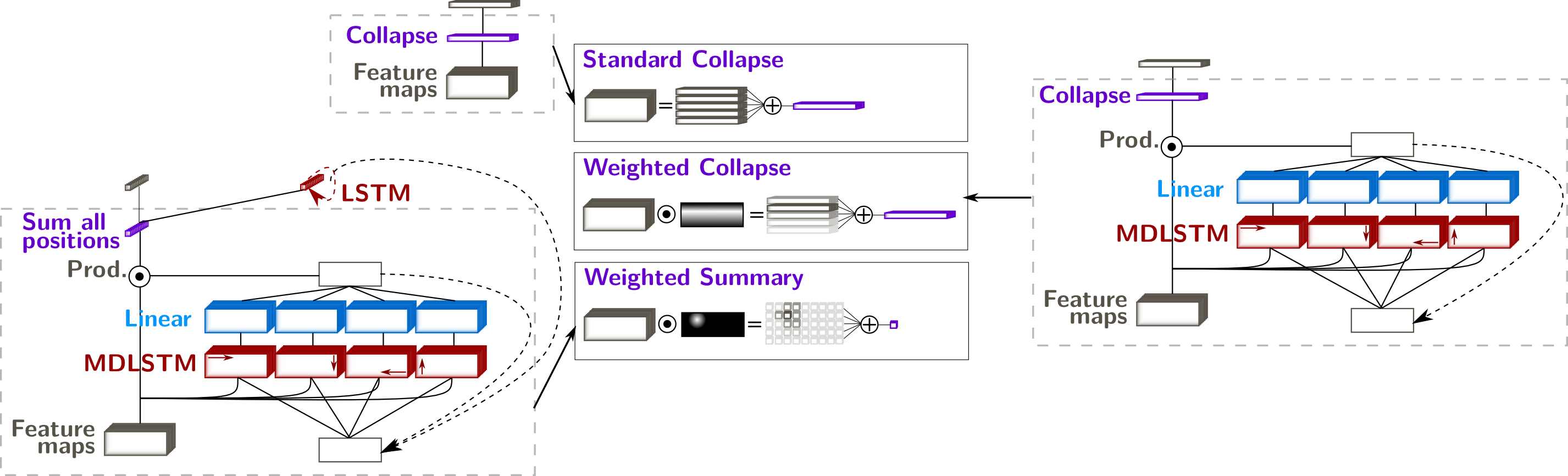
Weighted Summary - to predict one character at a time $$z_{t} = \sum_{i,j} \omega_{ij}^{(t)} e_{ij}$$
- the length of the output sequence is independent of the dimensions of the image
- at each timestep, a map of weights $\{\omega_{ij}^{(t)}\}$ is computed with a neural network
- the feature maps are multiplied by these weights, and summed to obtain one vector (summary) $z_t$
- the $t$-th character is predicted from vector $z_t$
Weighted Collapse - to recognize one line at a time $$z_{j}^{(t)} = \sum_{i=1}^H \omega_{ij}^{(t)} e_{ij}$$
- intermediate solution between the weighted summary and the standard collapse
- amounts to a standard collapse on the weighted sum
- the length of the $t$-th sequence is the width of the feature maps
- the weights are recomputed at each time step
- the $t$-th text line is recognized from sequence $z^{(t)}$
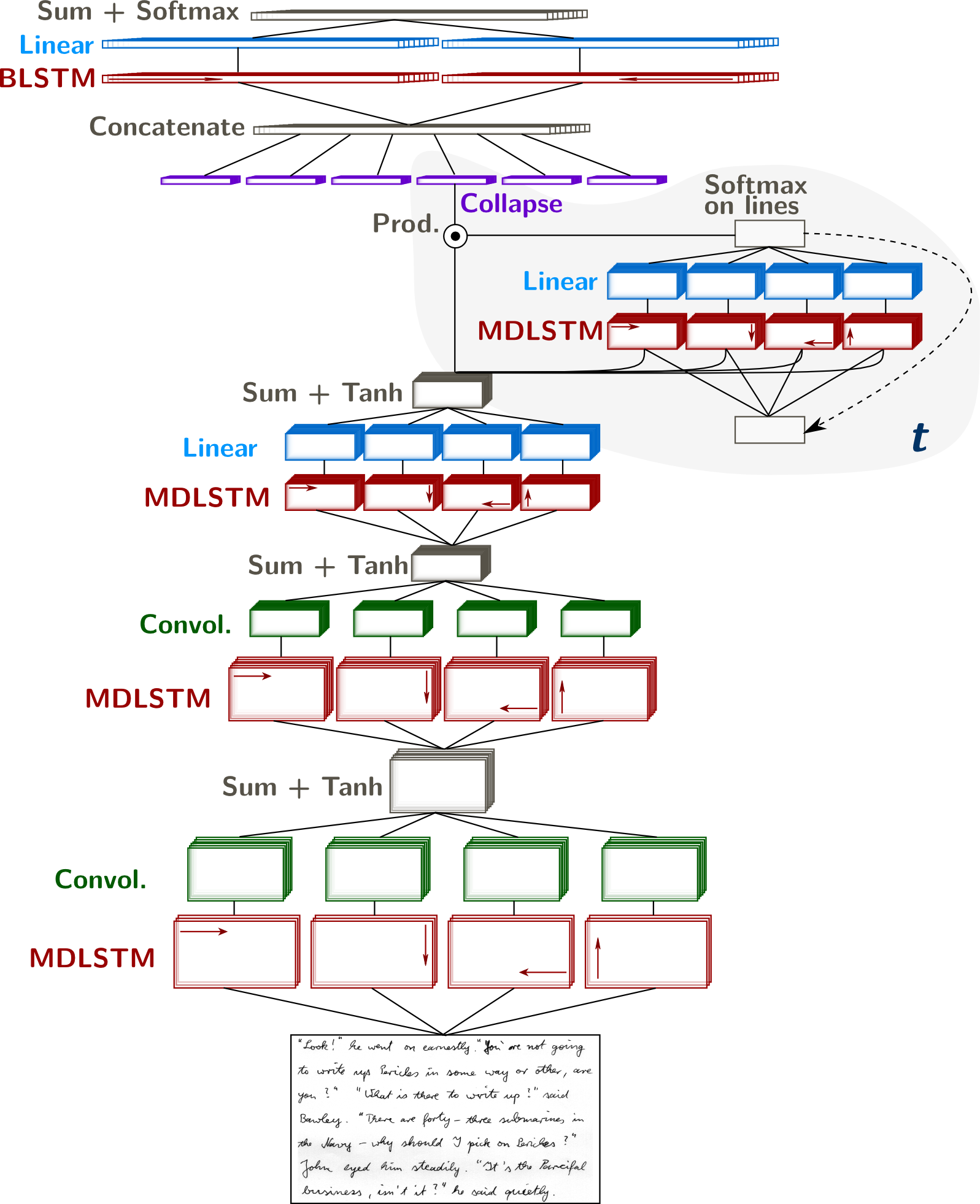
Scan, Attend and Read
In this model, a neural network computes a two-dimensional representation of the image. An "attention" neural network predicts where to focus in order to recognize the next character. It is a "soft attention" mechanism, which assign a score $\omega_{ij} \in [0,1]$, such that $\sum_{ij} \omega_{ij} = 1$ representing the probability of looking at position $(i,j)$ to recognize the next character. We use those weights in a weighted sum of the feature maps to predict the next character, as illustrated in the next figure.
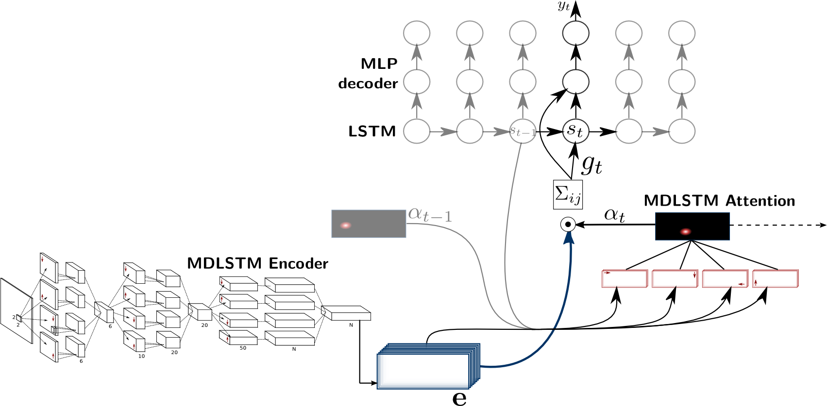
The proposed model comprises an encoder of the 2D image of text, producing feature maps, and a sequential decoder that predicts characters from these maps. The decoder proceeds by combining the feature vectors of the encoded maps into a single vector, used to update an intermediate state and to predict the next character in the sequence. The weights of the linear combination of the feature vectors at every timestep are predicted by the attention network.
System Overview
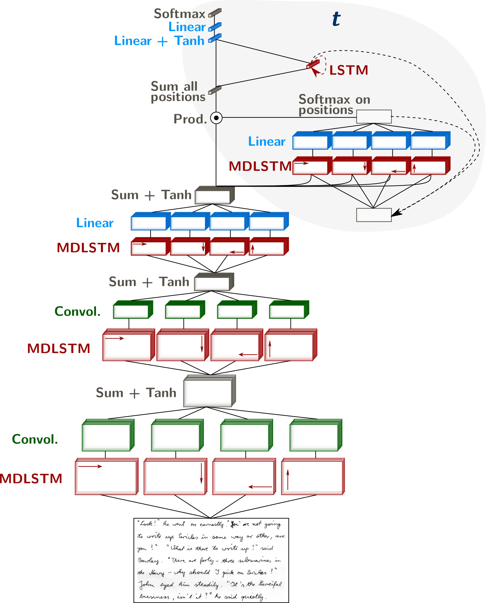
The classical MDLSTM network (except the collapse and softmax layers) is used as a feature extraction module, or encoder of the image $\mathcal{I}$: $$ e_{i,j} = Encoder( \mathcal{I} ) $$ where $(i,j)$ are coordinates in the feature maps
The attention mechanism provides a summary of the encoded image at each timestep in the form of a weighted sum of feature vectors. The attention network computes a score for the feature vectors at every position: $$ \omega_{ij}^{(t)} = Attention ( \mathbf{e}, \mathbf{\omega}^{(t-1)} , s_{t-1} ) $$ We refer to $\mathbf{\omega}^{(t)} = \{\omega_{ij}^{(t)}\}_{(1 \leq i \leq H,~1 \leq j \leq W)}$ as the attention map at time $t$, which computation depends not only on the encoded image, but also on the previous attention map, and on a state vector $s_{t-1}$.
In this model, we combine the previous attention map with the encoded features through an MDLSTM layer, which can keep track of position and content. With this architecture, the attention potentially depends on the context of the whole image. Moreover, the LSTM gating system allows the network to use the content at one location to predict the attention weight for another location. In that sense, we can see this network as implementing a form of both overt and covert attention. The attention map is the result of a softmax normalization of the output $\mathbf{m}$ of the MDLSTM attention network: $$ \omega_{ij}^{(t)} = \frac{e^{m_{ij}^{(t)}}}{ \sum_{i',j'} e^{ m_{i'j'}^{(t)} } } $$
The state vector $s_t$ allows the model to keep track of what it has seen and done. It is an ensemble of LSTM cells, whose inner states and outputs are updated at each timestep: $$ s_t = LSTM( s_{t-1}, z_t )$$ where $z_t$ represents the summary of the image at time $t$, resulting from the attention given to the encoder features: $$ z_t = \sum_{i,j} \omega_{ij}^{(t)} e_{i,j} $$ and is used both to update the state vector and to predict the next character.
The decoder predicts the next character given the current image summary and state vector: $$ y_t = Decoder( s_t, z_t ) $$ Here, the decoder is a simple multi-layer perceptron with one hidden layer ($\tanh$ activation) and a softmax output layer.
Modification of the MDLSTM for Attention
Compared to the standard LSTM, there is one weight vector $\rho_\bullet$ for each gate scaling the previous attention and one weight matrix $\mathbf{\kappa}_\bullet$ for each gate scaling the previous state vector.
Input Gate $$ z^{i,j}_\iota = f({\color{blue}\rho_\iota \alpha_{t-1}^{ij} + \sum_{l=1}^S \kappa_{l\iota} s_{t-1,l} } + \sum_{i=1}^I w_{i\iota}x_i^{i,j} + \sum_{h=1}^H w_{h\iota} z_h^{i-1,j} + w_{h\iota'} z_h^{i,j-1}) $$ Forget Gates $$ z^{i,j}_{\phi_1} = f({\color{blue}\rho_\phi \alpha_{t-1}^{ij} + \sum_{l=1}^S \kappa_{l\phi} s_{t-1,l} } + \sum_{i=1}^I w_{i\phi}x_i^{i,j} + \sum_{h=1}^H w_{h\phi} z_h^{i-1,j} + w_{h\phi'} z_h^{i,j-1}) $$ $$ z^{i,j}_{\phi_2} = f({\color{blue}\rho_{\phi'} \alpha_{t-1}^{ij} + \sum_{l=1}^S \kappa_{l\phi'} s_{t-1,l} } + \sum_{i=1}^I w_{i\phi}x_i^{i,j} + \sum_{h=1}^H w_{h\phi} z_h^{i-1,j} + w_{h\phi'} z_h^{i,j-1} ) $$ Output Gate $$ z^{i,j}_\omega = f( {\color{blue}\rho_\omega \alpha_{t-1}^{ij} + \sum_{l=1}^S \kappa_{l\omega} s_{t-1,l} } + \sum_{i=1}^I w_{i\omega} x_i^{i,j} + \sum_{h=1}^H w_{h\omega} z_h^{i-1,j} + w_{h'\omega} z_h^{i,j-1} ) $$ Cell state $$ a^{i,j}_c = {\color{blue}\rho_c \alpha_{t-1}^{ij} + \sum_{l=1}^S \kappa_{lc} s_{t-1,l} } + \sum_{i=1}^I w_{ic} x_i^{i,j} + \sum_{h=1}^H w_{hc} z_h^{i-1,j} + w_{hc'} z_h^{i,j-1} $$ $$ s^{i,j}_c = z^{i,j}_{\phi_1} s^{i-1,j}_c + z^{i,j}_{\phi_2} s^{i,j-1}_c + z^{i,j}_\iota g(a^{i,j}_c) $$
Training
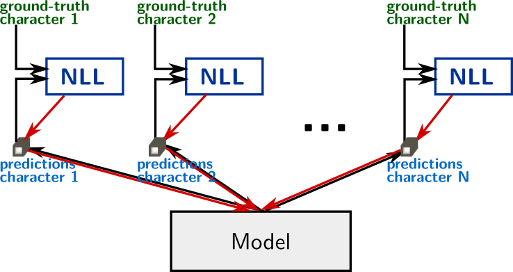
The neural network computes a fully differentiable function, which parameters can be trained with backpropagation. The optimized cost is the negative log-likelihood of the correct transcription: $$ \mathcal{L}(\mathcal{I}, \mathbf{y}) = - \sum_{t} \log p(y_t | \mathcal{I}) $$ where $\mathcal{I}$ is the image, $\mathbf{y}=y_1,\cdots,y_T$ is the target character sequence and $p( \cdotp | \mathcal{I})$ are the outputs of the network.
In addition to characters, we include a special token EOS at the end of the target sequences. This token is also predicted by the network to indicate when to stop reading at test time. Moreover, there is no "blank" token as in CTC.
Training tricks
In order to get the model to converge, or to converge faster, a few tricks helped:
- Pretraining use an MDLSTM network (no attention) trained on single lines with CTC as a pretrained encoder
- Data augmentation add to the training set all possible sub-paragraphs (i.e. one, two, three, ... consecutive lines)
- Curriculum (0/2) training the attention model on word images or single line images works quite well, do this as a first step
- Curriculum (1/2) (Louradour et al. ,2014) draw short paragraphs (1 or 2 lines) samples with higher probability at the beginning of training
- Curriculum (2/2): incremental learning. Run the attention model on the paragraph images N times (e.g. 30 times) during the first epoch, and train to output the first N characters (don't add EOS here). Then, in the second epoch, train on the first 2N characters, etc.
- Truncated BPTT to avoid memory issues
Results
Text Line Recognition
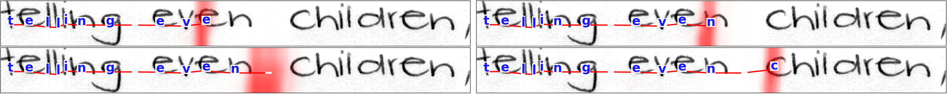
First, we trained the network on text lines with several words (i.e. usual task). In the following picture, we see that the network learnt to focus on successive characters.
Learning Line Breaks
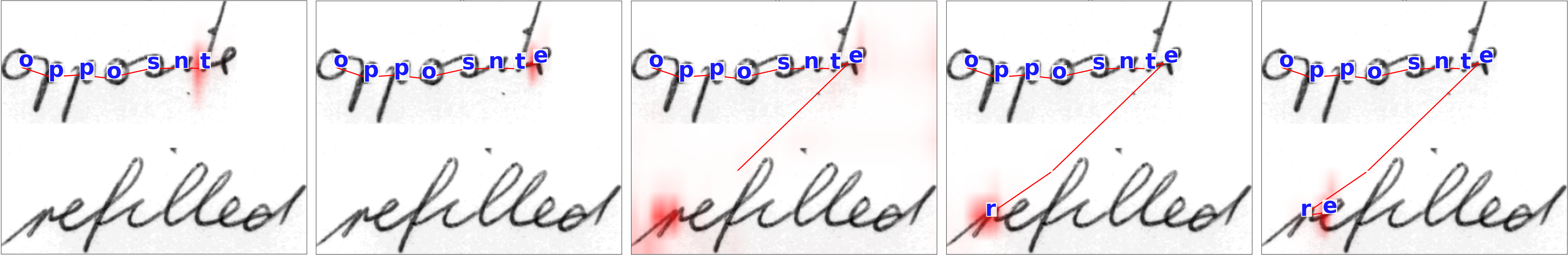
For end-to-end recognition of complete paragraphs, we need the network to be able to look for the next line. As a toy experiment, we created a syntetic dataset of images of two stacked words (from the IAM database). We did not include a newline symbol. In the example below, the target character sequence would be "opposite refilled". We see that in that context, the network was able to go to the next line.
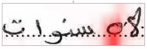
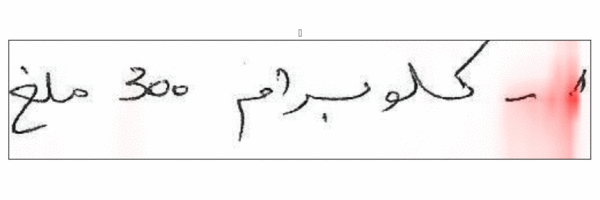
Bi-directional Scripts
Arabic, for example, is written (and read) from right to left. However, numbers, or some foreign words are still read left-to-right. With a sliding window approach, or with CTC, the targets (and predictions) should be very carefully pre-processed (respectively post-processed) to take into account this bi-directionality. We trained the same model as above, without any modification, on an Arabic database containing a small amount of cases with mixed reading orders (and a lot of examples with only Arabic). In the next animation, we see that the model not only learnt that Arabic is written right-to-left, but it can also handle bi-directional text.
 |
 |
Paragraph Recognition
The following video shows the model (trained on full paragraphs) transcribing paragraphs.
Intermediate Activations
As promised, here are the activations of the same layers, for the same paragraph image as previously, but with a training on paragraphs with the attention model. We see that they are much better than those of the MDLSTM trained with collapse and CTC, and let us think that they could be re-used for other tasks.
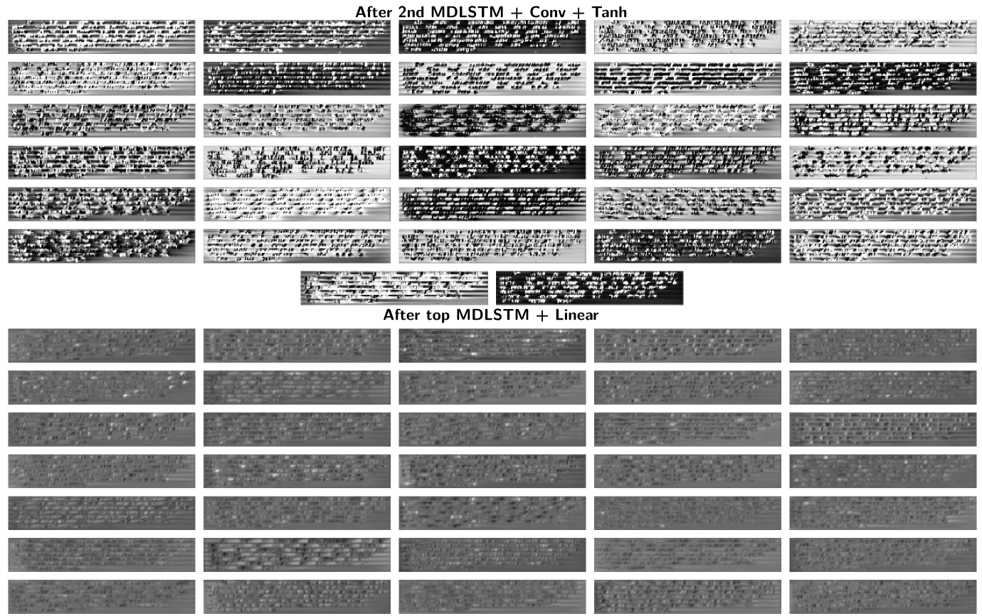
Intermediate Activations of the Attention Model
Pros & Cons
- Can potentially handle any reading order
- Can output character sequence of any length
- Can recognize paragraphs (and maybe complete document?)
- Very slow (one fprop in the attention network and decoder for each character = about 500 times for a complete paragraph)
- Requires a lot of memory during training (same reasons)
- Not quite close to state-of-the-art performance on paragraphs (for now...)
Attention on Text Lines: Joint Line Segmentation and Transcription
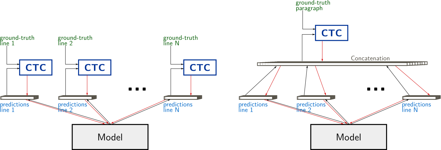
$ \newcommand{\ijt}[3]{#1_{#2}^{(#3)}} $The main issue with the previous model is speed. The attention should be recomputed for each character, that is about 500 times. Transcribing a whole paragraph takes about 20 sec, when the line-level MDLSTM do it in less than 1 sec. The next model combines the attention mechanism (which allows to handle full paragraphs) with the collapse layer for quick line-level recognition. In this model, the attention is put on lines, and computed only once for each line, yielding processing times that are close to the baseline system.
System Overview
As before, the classical MDLSTM network (except the collapse and softmax layers) is used as a feature extraction module, or encoder of the image $\mathcal{I}$: $$ e_{i,j} = Encoder( \mathcal{I} ) $$ where $(i,j)$ are coordinates in the feature maps
In this model, we replace the simple sum of the collapse layer by a weighted sum, in order to focus on a specific part of the input. The weighted collapse is defined as follows: $$ \ijt{z}{j}{t} = \sum_{i=1}^H \ijt{\omega}{ij}{t} e_{ij} $$ where $\ijt{\omega}{ij}{t}$ are scalar weights between $0$ and $1$, computed at every time $t$ for each position $(i,j)$. The weights are provided by a recurrent neural network, enabling the recognition of a text line at each timestep. This collapse, weighted with a neural network, may be interpreted as the attention module. $$ \ijt{\omega}{ij}{t} = Attention ( \mathbf{e}, \mathbf{\omega}^{(t-1)} ) $$ The main difference with the attention of the previous model is the softmax normalization, done columnwise here instead of over the whole map. If $\mathbf{m}$ is the output of the MDLSTM attention network: $$ \omega_{ij}^{(t)} = \frac{e^{m_{ij}^{(t)}}}{ \sum_{i'} e^{ m_{i'j}^{(t)} } } $$ Note also that we did not use a state vector in this model.
This module is applied several times to the features from the encoder. The output of the attention module at iteration $t$ is a sequence of feature vectors $\mathbf{z}$, intended to represent a text line. Therefore, we may see this module as a soft line segmentation neural network.
A decoder predicts a character sequence from the feature vectors: $$ \mathbf{y} = Decoder( \mathbf{z} ) $$ where $\mathbf{z}$ is the concatenation of $z^{(1)}, z^{(2)}, \ldots, z^{(T)}$. Alternatively, the decoder may be applied to $z^{(i)}$s sub-sequences to get $y^{(i)}$s and $\mathbf{y}$ is the concatenation of $y^{(1)}, y^{(2)}, \ldots, y^{(T)}$. The decoder is a Bidirectional LSTM (BLSTM) processing the whole paragraph, which can model dependencies across text lines.
Training
Training this model turned out to be much easier than the previous one. We started with the same pre-trained encoder. We did not do any data augmentation. The only curriculum was to first train one epoch on paragraphs of two lines to initiate the attention network. We did not have to truncate the BPTT to avoid memory issues.
We trained the model with the CTC objective function. When the line breaks are known in the annotation, we can apply the CTC to the output segments corresponding to line segments (i.e. one timestep of the attention module). However, we chose the scenario of unknown line breaks and applied CTC to the whole paragraph directly.
Results
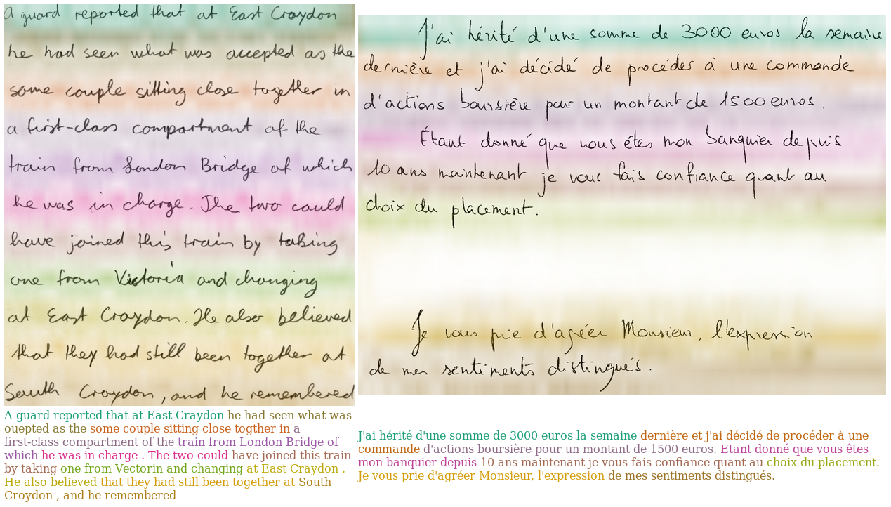
In the following figure, we show, for two paragraphs:
- The attention weights in different colors for different timesteps, which may be interepreted as an implicit line segmentation
- The output of the network (text below the images) with colors corresponding to the different timesteps of the attention module
Pros & Cons
- Much faster then "Scan, Attend and Read"
- Easier paragraphs training
- Results are competitive with state-of-the-art models
- The attention spans the whole image width, so the method is limited to paragraphs (not full, complex, documents)
- The reading order is not learnt
Final Word
We presented two models, based on learnt attention mechanisms, to recognize the handwritten text in images of paragraphs, without prior nor explicit line segmentation, in an end-to-end manner, with neural networks. We displayed quantitative results of these models. For the details on the architecture of the networks, training parameters, and quantitative results, please refer to the papers. Do not hesitate to contact me (firstname dot surname at gmail) if you want to know more, or if you have questions.
References
... soon ... please refer to the papers for now ...
Copyright Notice.This material is presented to ensure timely dissemination of scholarly and technical work. Copyright and all rights therein are retained by authors or by other copyright holders. All persons copying this information are expected to adhere to the terms and constraints invoked by each author's copyright. These works may not be reposted without the explicit permission of the copyright holder.