The intriguing blank label in CTC
Théodore Bluche, Christopher Kermorvant, Hermann Ney, Jérôme Louradour
Abstract
In recent years, Long Short-Term Memory Recurrent Neural Networks (LSTM-RNNs) trained with the Connectionist Temporal Classification (CTC) objective won many international handwriting recognition evaluations. The CTC algorithm is based on a forward-backward procedure, avoiding the need of a segmentation of the input before training. The network outputs are characters labels, and a special non-character label. On the other hand, in the hybrid Neural Network / Hidden Markov Models (NN/HMM) framework, networks are trained with framewise criteria to predict state labels. In this paper, we show that CTC training is close to forward-backward training of NN/HMMs, and can be extended to more standard HMM topologies. We apply this method to Multi-Layer Perceptrons (MLPs), and investigate the properties of CTC, especially the role of the special label.
Acknowledgements. This work was carried out during my PhD in the research team of A2iA and at the LIMSI-CNRS lab, under the supervision of Prof. Hermann Ney (RWTH Aachen, LIMSI) and Christopher Kermorvant (Teklia, A2iA). Please cite one of the following if you wish to refer to this work:
- Théodore Bluche, Christopher Kermorvant, Hermann Ney, Jérôme Louradour (2016) La CTC et son intrigant label "blank" - Étude comparative de méthodes d'entraînement de réseaux de neurones pour la reconnaissance d'écriture In Colloque International Francophone sur l'Ecrit et le Document (CIFED), to appear.
- Théodore Bluche (2015) Deep Neural Networks for Large Vocabulary Handwritten Text Recognition. PhD thesis. Chap. 7.
- Théodore Bluche, Hermann Ney, Jérôme Louradour, Christopher Kermorvant (2015) Framewise and CTC Training of Neural Networks for Handwriting Recognition. In 13th International Conference on Document Analysis and Recognition (ICDAR), 81-85.
Introduction
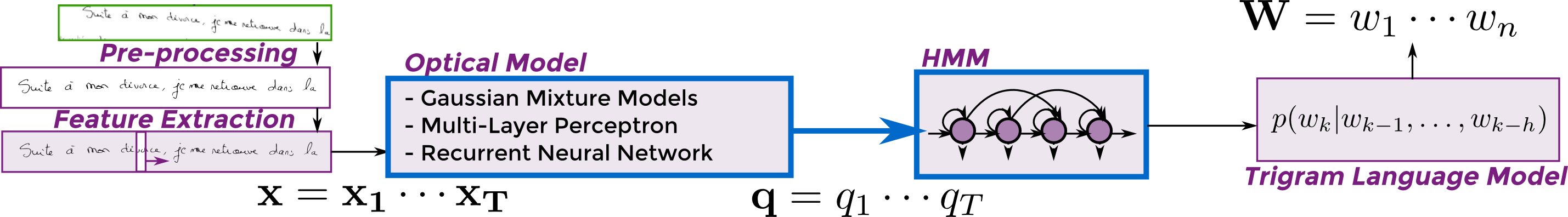 |
- We are interested in the hybrid (R)NN/HMM framework where the network predicts HMM states
- Some works in the '90s for integrated NN/HMM training
- Today, mostly framewise training from forced alignments, or CTC with RNNs
Questions:
- What are the differences bewteen framewise, CTC, and integrated training ?
- Can we apply CTC to other neural nets than RNNs ?
- Can we use the CTC paradigm with other targets than characters and blank (e.g. HMM states) ?
- What is the role of the blank symbol in CTC? How and when does it help ?
NB. Some useful references for intergrated NN/HMM training: [Bengio et al., 1992, Haffner, 1993, Senior and Robinson, 1996, Konig et al., 1996, Hennebert et al., 1997, Yan et al., 1997], and for CTC: [Graves et al., 2006]
Relation between CTC and integrated NN/HMM training
The equations are in the paper(s). Basically:
CTC = HMM training, without transition/prior probabilities
(zeroth-order model), and with specific outputs for standalone NN recognition ( = one HMM state / char. + blank)
CTC could be applied with different HMM topologies, to other kinds of NN than RNN (e.g. MLPs)
CTC = Cross-entropy training + forward-backward to consider all possible segmentations
we can compare the training strategies, see the effect of forward-backward,
with different HMM topologies (number of HMM states / char.)
The differences are summarized in the following table:
| Training | Cost | NN outputs |
|---|---|---|
| Cross-entropy | $$-\log \prod_t P(q_t | x_t)$$ | HMM states (5-6 / char.) |
| CTC | $$-\log {\color{myblue} \sum_{\mathbf{q}}} \prod_t P(q_t | \mathbf{x})$$ | characters + blank |
| HMM training | $$-\log {\color{myblue} \sum_{\mathbf{q}}} \prod_t \frac{P(q_t | x_t)}{\color{myred} P(q_t)} {\color{myred} P(q_t | q_{t-1})}$$ | HMM states (5-6 / char.) |
Experimental comparison between CTC and framewise training
Experimental Setup
Goal: study the differences and dynamics of training methods
- IAM database : 6.5k lines for training, results reported on validation set of 976 lines
- Image pre-processing
- skew and slant correction [Buse et al., 1997]
- contrast enhancement
- height normalization
- Feature extraction
- Sliding window of 3px scanned left-to-right with no overlap
- Extraction of 56 geometrical and statistical features [Bianne et al., 2011]
- Hybrid NN/HMM systems using scaled NN posteriors $p(q_t|x_t) / p(q_t)$
- Trigram language model with vocabulary of 50k words (trained on LOB, Brown and Wellington corpora), ppl 298, OOV 4.3%
- FST-based decoder of the KALDI toolkit
- Small Neural Nets for fast experiments
- MLP with 2 sigmoid hidden layers of 1,024 units
- BLSTM-RNNs with one hidden layer of 100 LSTM units in each direction
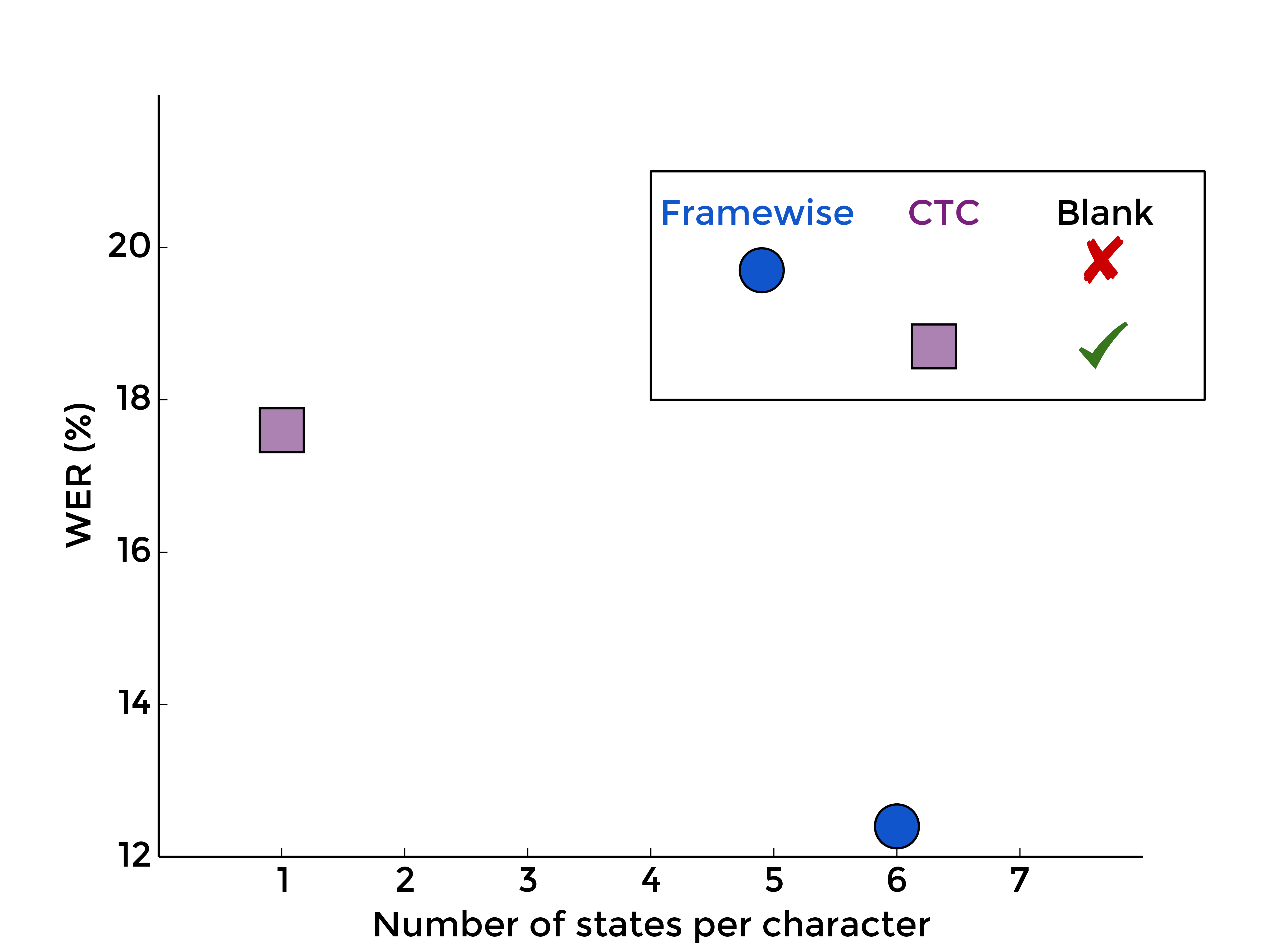
Framewise and CTC training: impact of number of states and blank label
1. The usual comparison
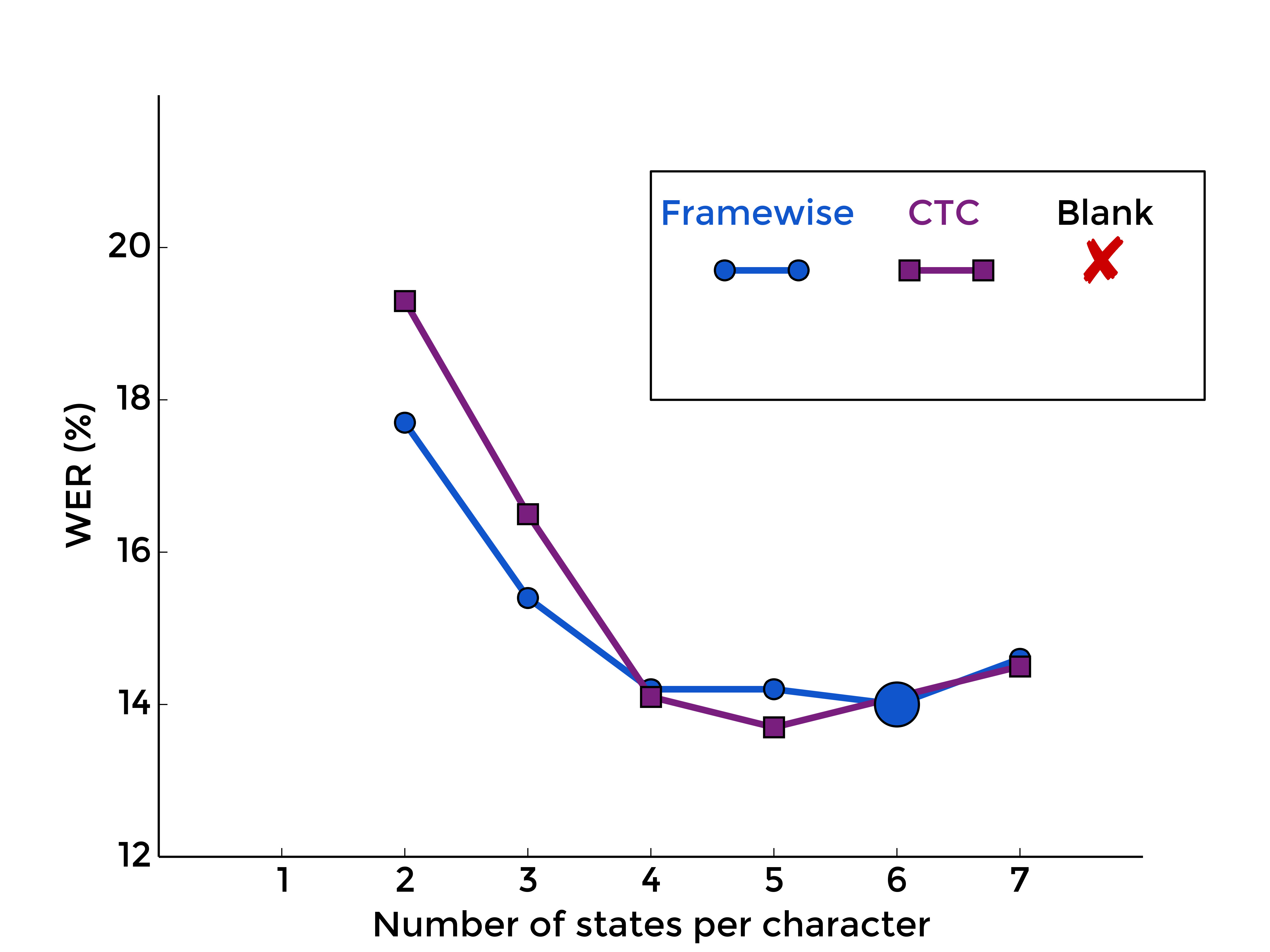
First, let's do the usual comparison, the one you will find in many papers switching from classical framewise training from HMM alignments to CTC. We compare on the one hand the framewise system, with standard multi-state without blank HMMs, and on the other hand CTC as defined in [Graves et al., 2006], with one-state character models, and blank:
 |
 |
| MLP | RNN |
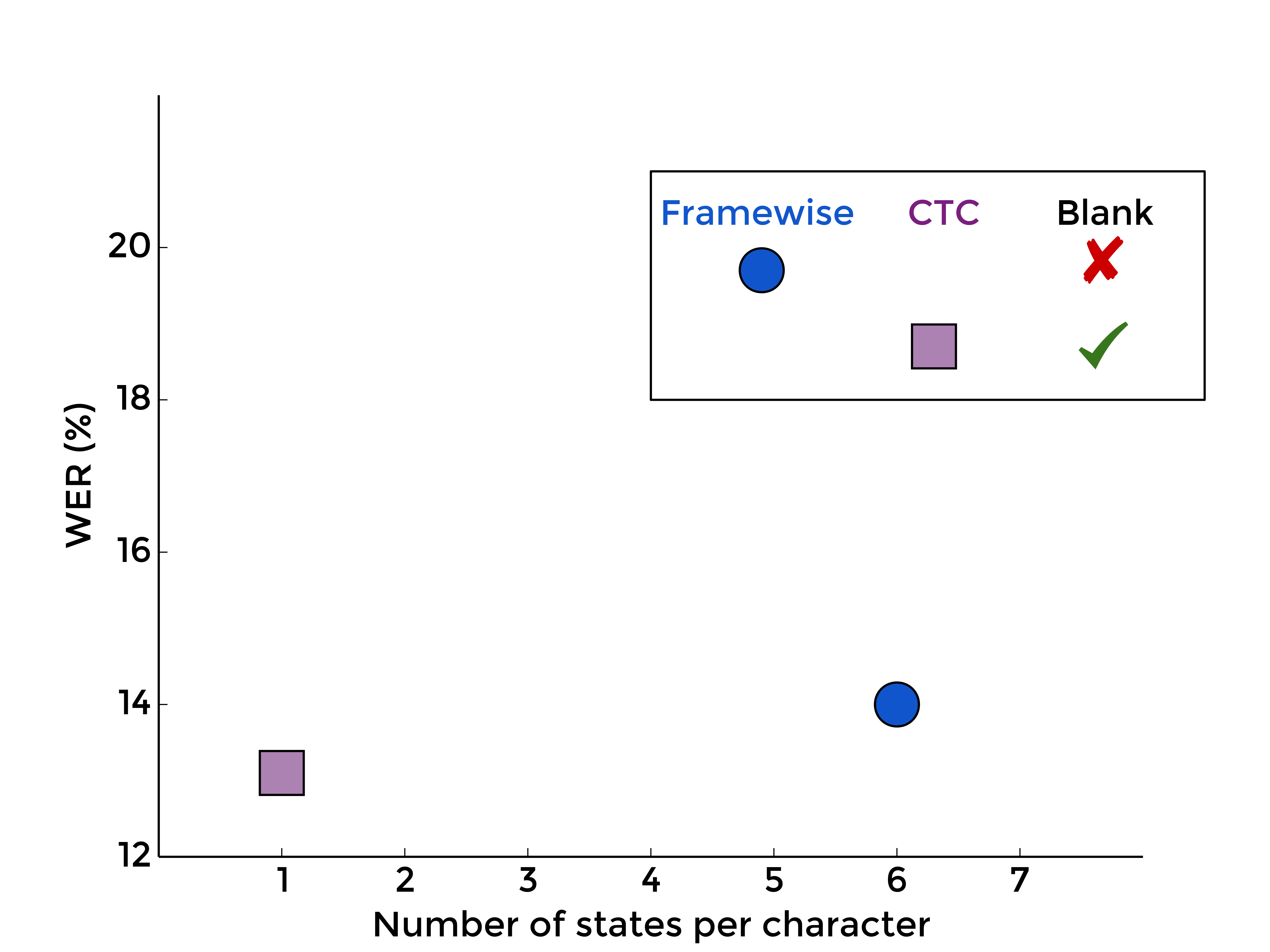
2. Summing over all labelings
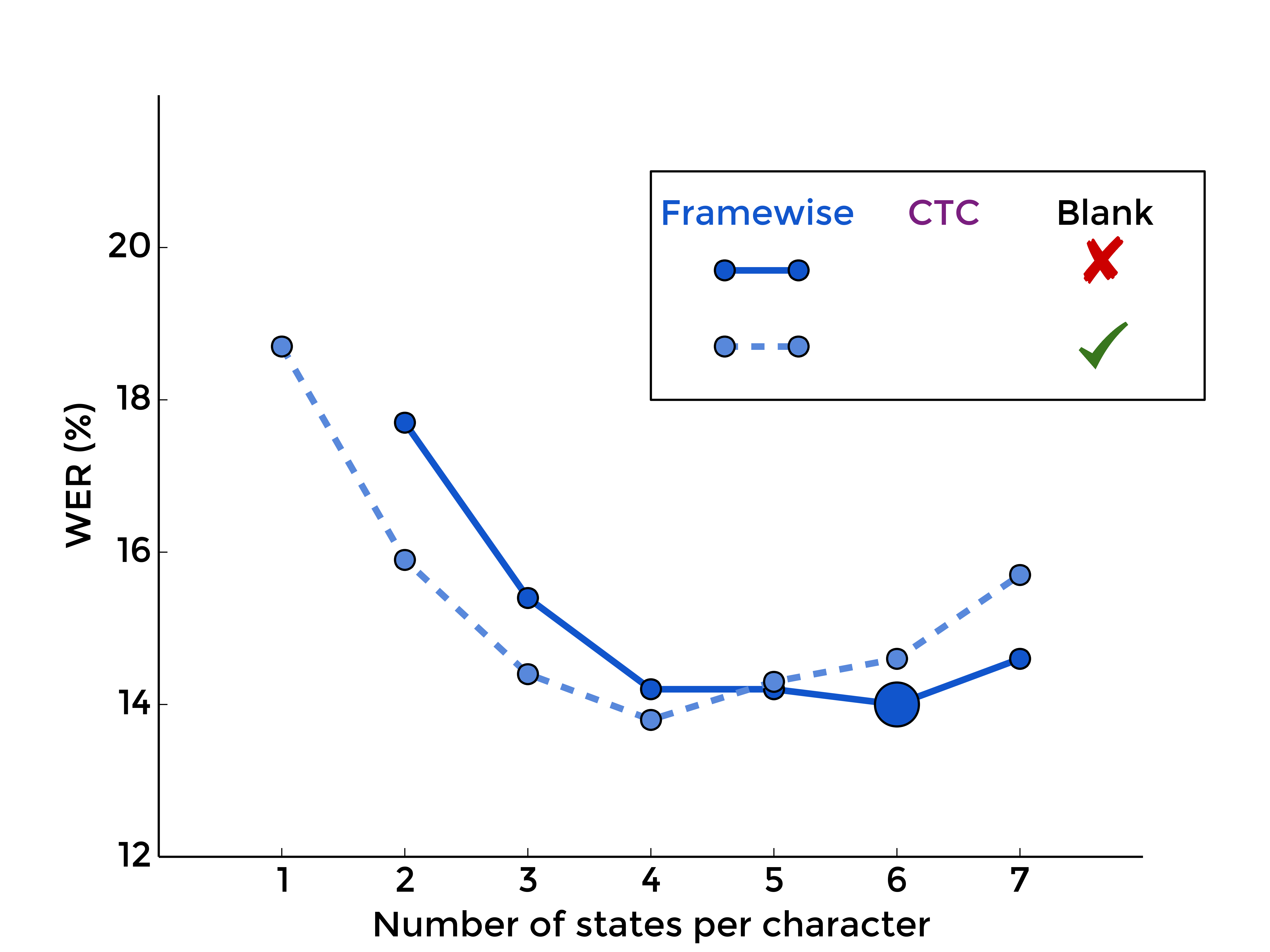
One of the aspect of CTC, the one most visible in the cost function, is the segmentation-free approach by summing over all possible labelings. Let's forget about blank and evaluate only this aspect with different numbers of states per character:
 |
 |
| MLP | RNN |
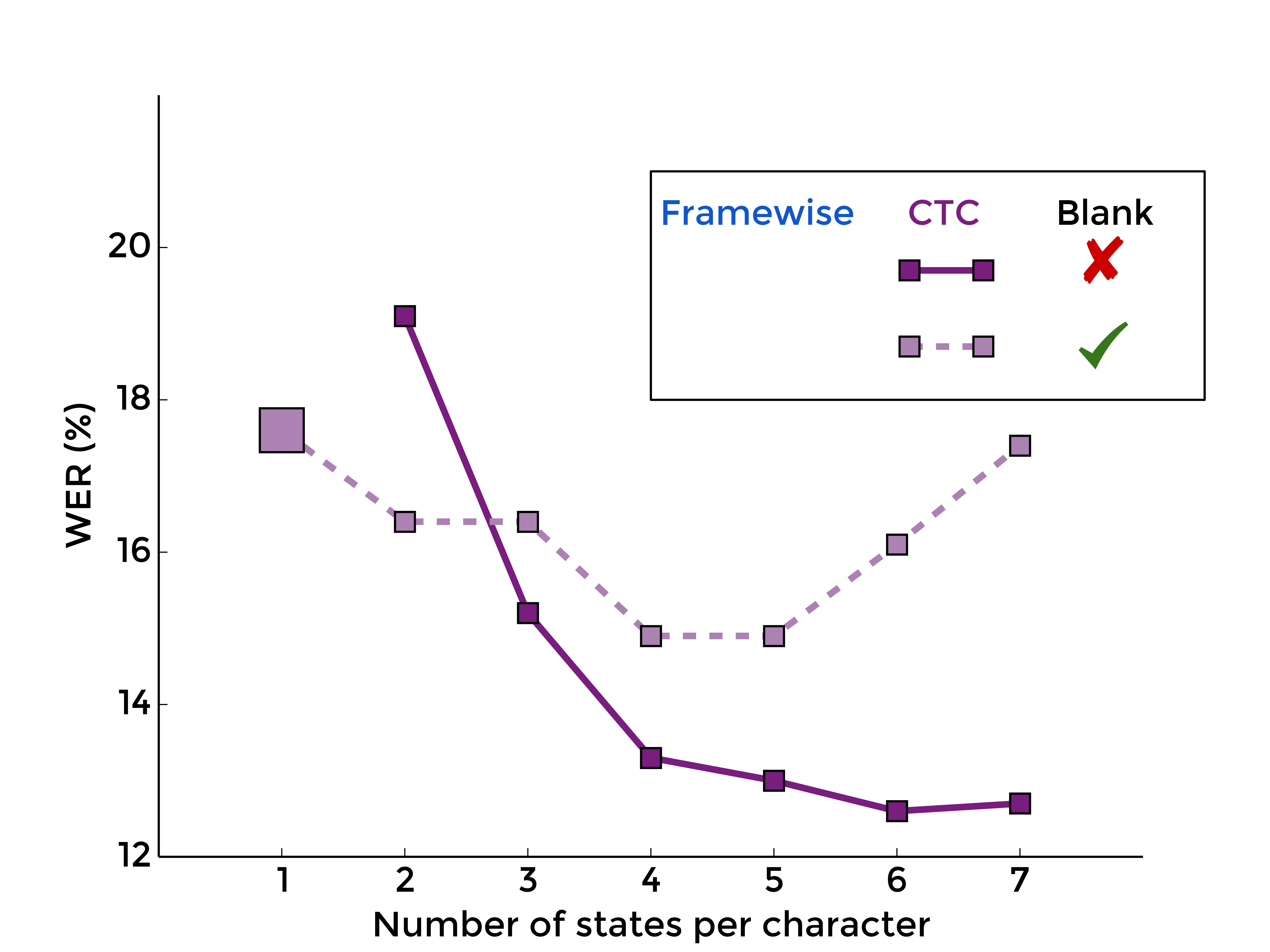
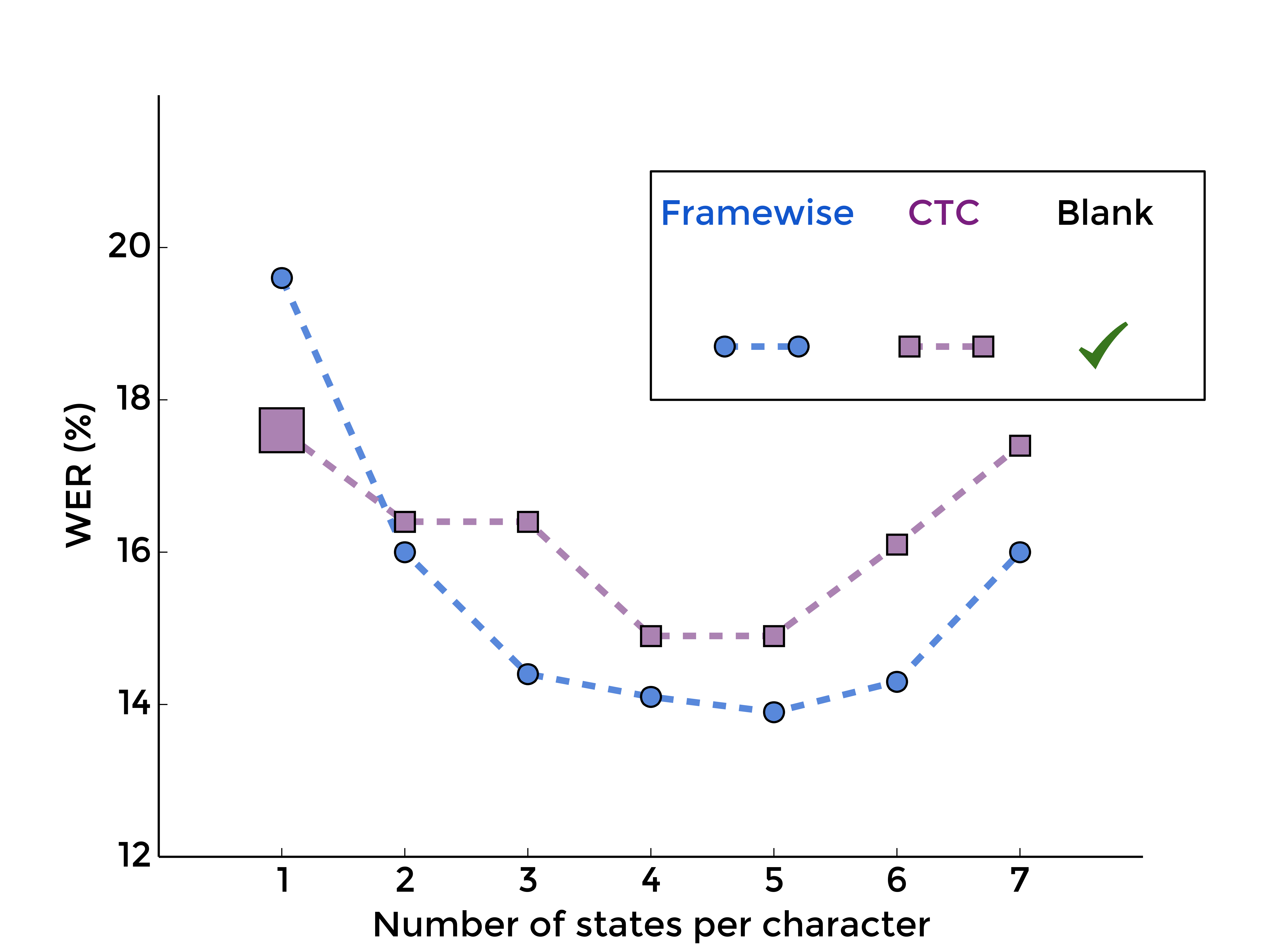
3. The Blank Label
Back to the blank label, let's see what is the effect of optionaly adding it between every character model, with framewise training first, and with CTC-like training, for different numbers of states per characters:
 |
 |
| MLP | RNN |
 |
 |
| MLP | RNN |
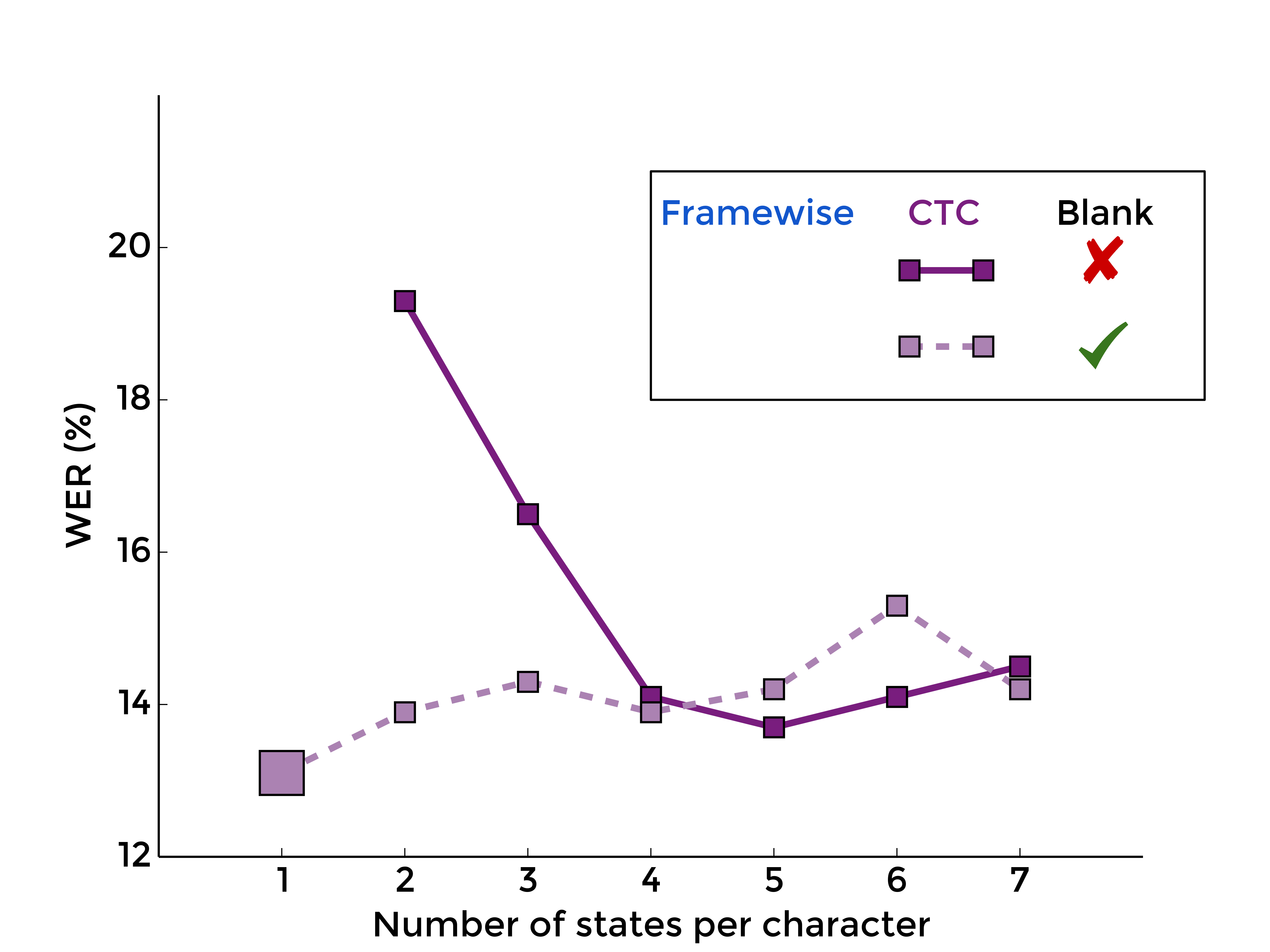
4. Summing over all labellings with blank
To complete the picture, we may also evaluate the segmentation-free aspect of CTC when the blank label is included:
 |
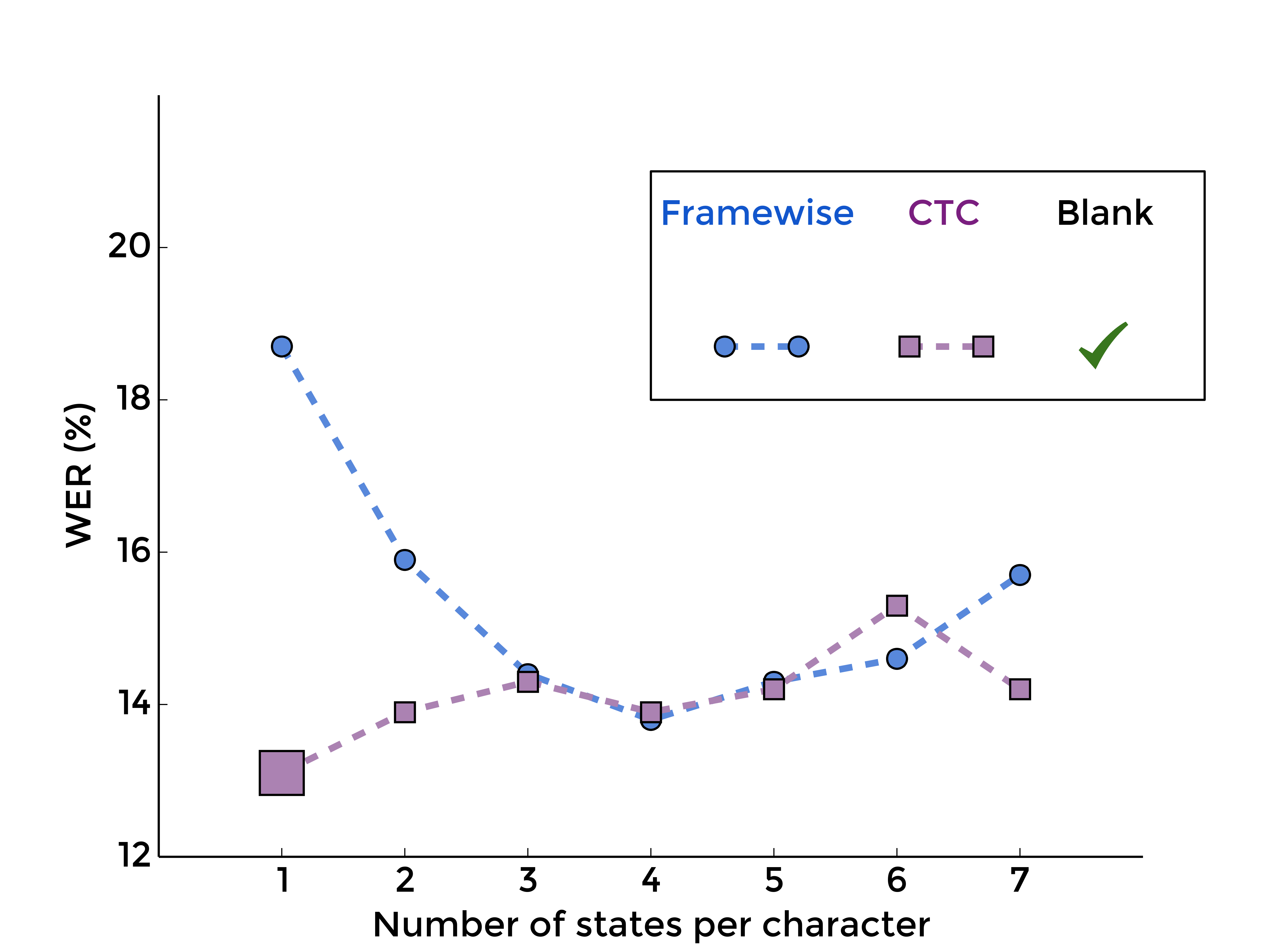 |
| MLP | RNN |
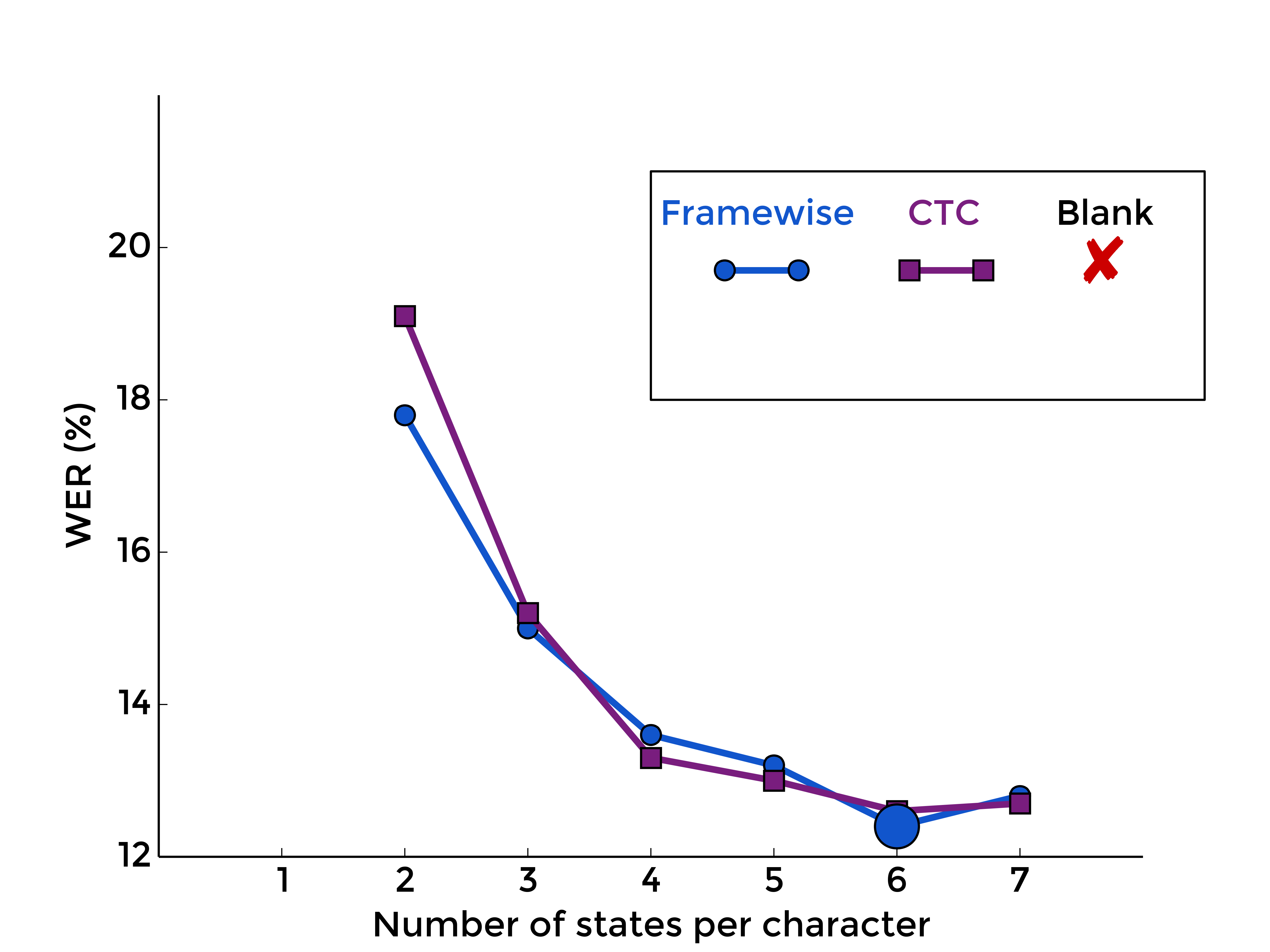
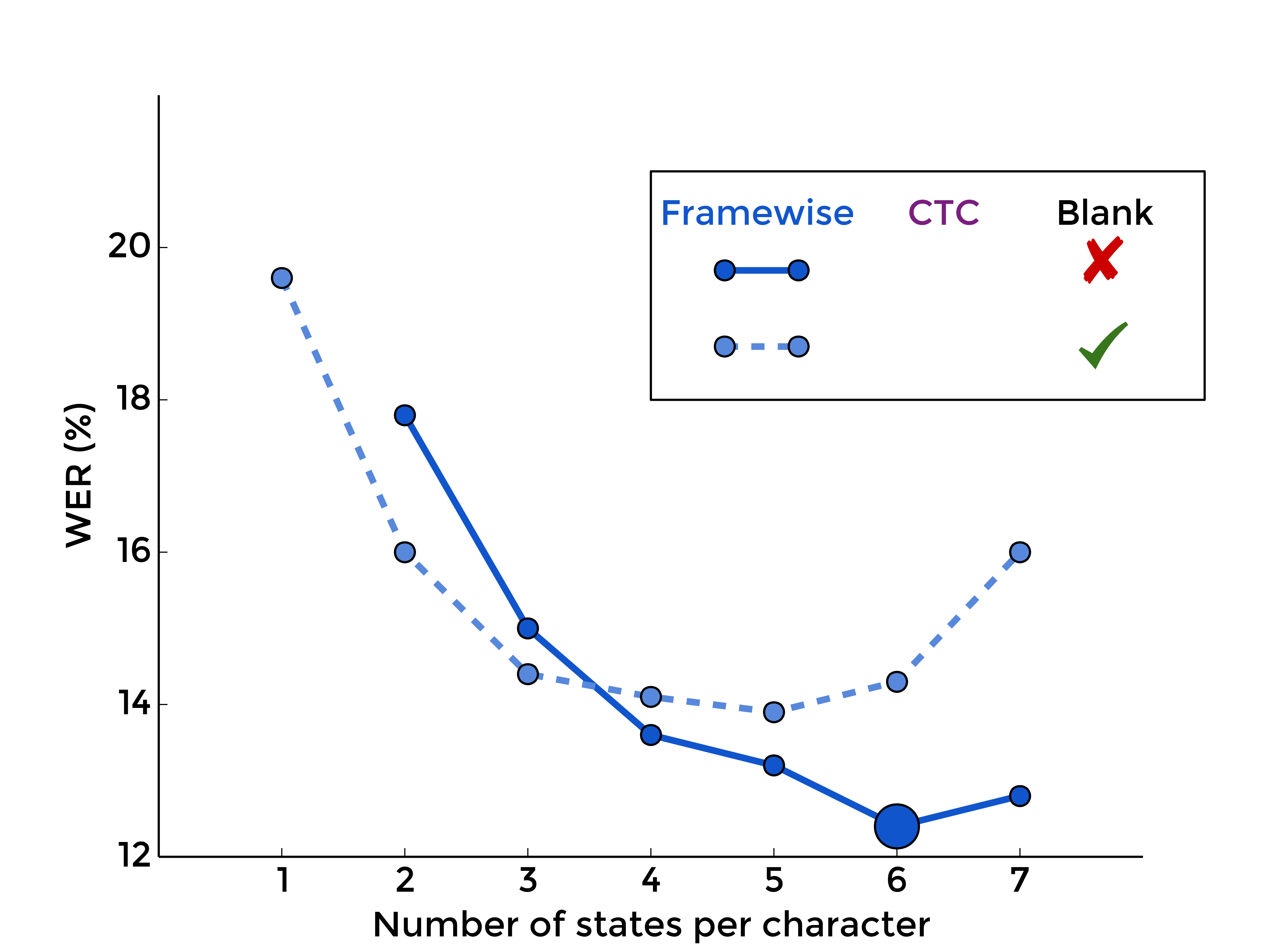
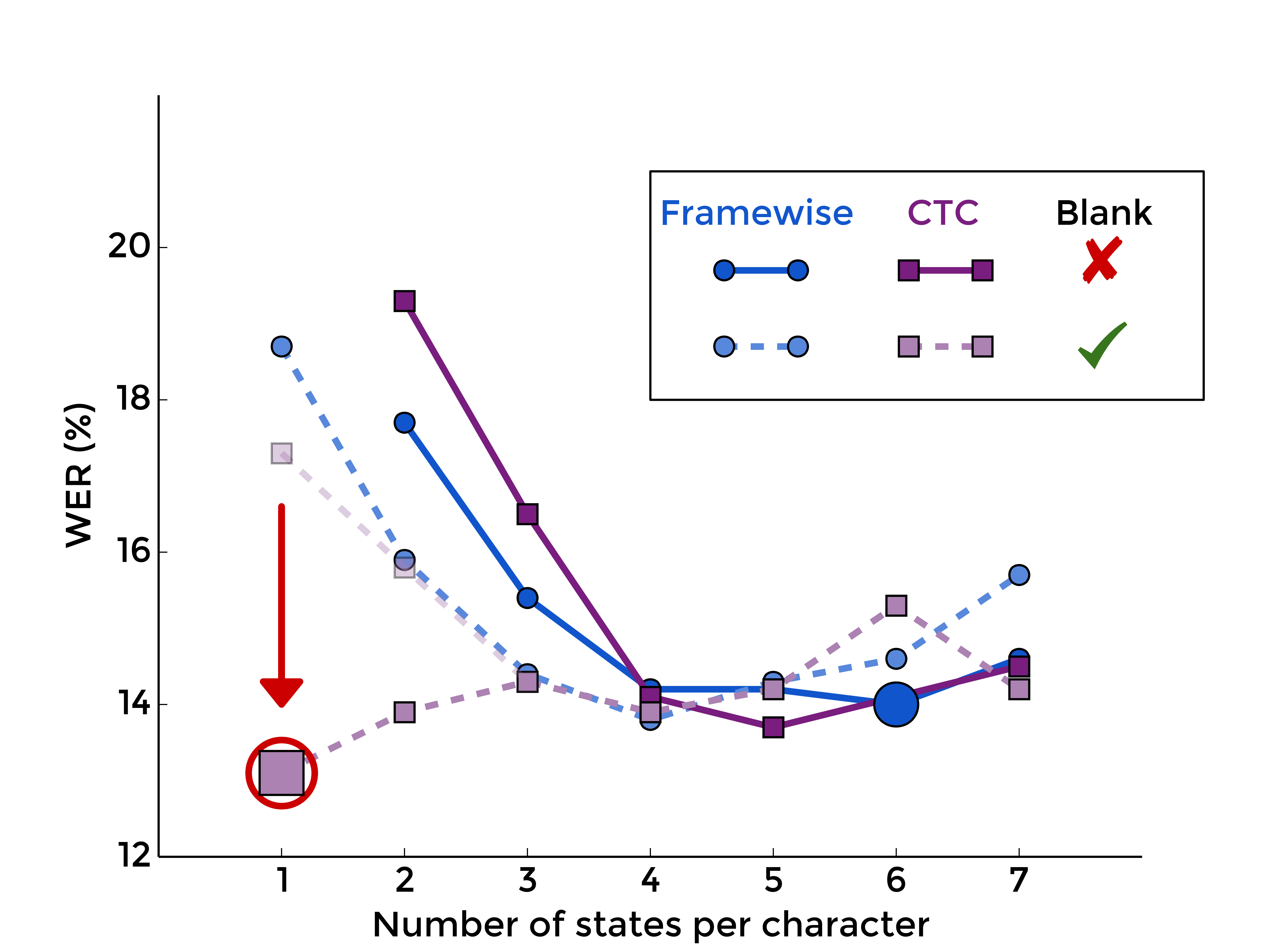
5. Summary
Merging all these plots, we can see that more or less all curves, i.e. all choices of blank inclusion and training method, look practically the same, except for one:
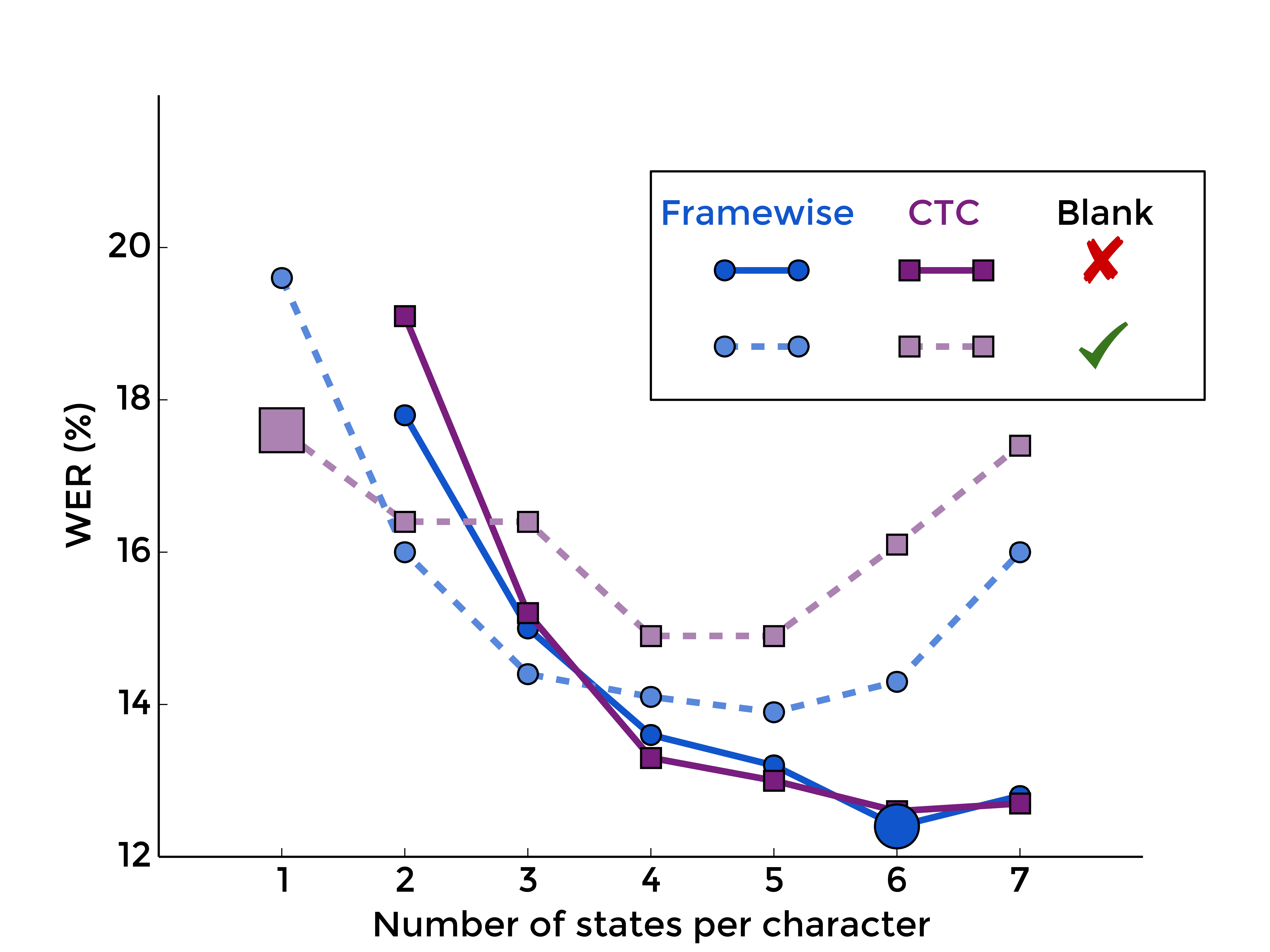 |
 |
| MLP | RNN |
Interaction between CTC and blank
Peaks
A typical observation in CTC-trained RNNs is the dominance of blank predictions in the output sequence, with localized peaks for character predictions. Interestingly, this behaviour still occurs with more states (e.g. with three states: three peaks of states predictions with many blanks between each character). We also observe this with CTC-trained MLPs. Thus, we can conclude that this typical output is due to the interaction between blank and CTC training, rather than a consequence of using RNNs or single-state character models.
On the following figure, we show how the outputs of a network with one state per character and blank evolve in the beginning of CTC training. In the top left plot, we see the outputs before training. Since the weights of the network have not yet been adjusted, the outputs are more or less random. As the training procedure advances, the predictions of the blank symbol increases, until the posterior probability is close to one for the whole sequence (end of the second line). At this point, the network predicts only blank labels. Then (third line), the probabilities of character labels start increasing, and peaks emerge at specific locations.
This is not surprising. In the CTC graph, there is one blank between each character. In early stages of training, the NN outputs are more or less random (at first approximation, drawn from a uniform distribution). Any path is equally likely, but summing all blank posteriors for a given timestep in the forward-backward procedure, the target for blank will be much higher than for any other character. The backpropagated error will make the network more likely to give a high posterior probability to the blanks, which in turn will favor path with many blanks in subsequent forward-backward computations of the cost.
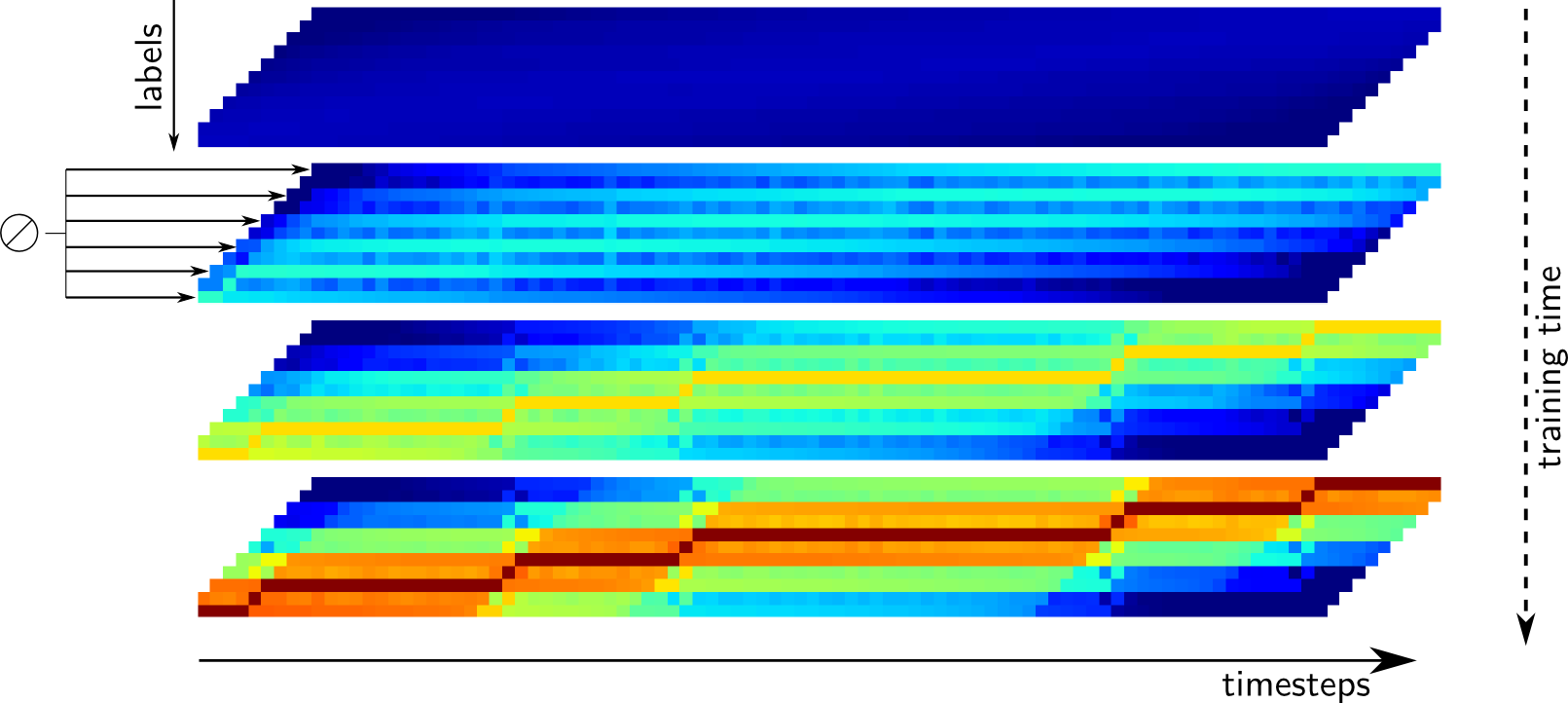 |
The previous figure shows the posterior probabilities computed with the forward-backward algorithm during training, which are the targets of the CTC training algorithm. We see that the fact that one in two labels is a blank will give a higher posterior probability for this symbol. When the network starts outputting only blanks, the paths with many blanks will be more likely. On the other hand, the difference between the network output for the blank label, and the posterior probability of the blank computed with the forward-backward algorithm will become small.
Predicting only blanks will penalize the cost function because of the low probabilities given to characters, and the network has only to find one location to predict each character, to "jump" from one sequence of blanks to another. Since a valid path must go through character labels, the posterior probabilities of these labels will also increase. We see on the second plot of the previous figure that at some positions, the character labels have a higher posterior probability. Since the network predicts only blanks, the gradients for characters at these positions will be high, and the network will be trained to output the character labels at specific locations. Finally, the path with blanks everywhere and characters at localized position will have a much higher probability, and the training algorithm may not consider much the other possible segmentations (bottom plot of the previous figure).
What happens without blank?
Actually, the results of CTC without blank presented previously were not trained with CTC from scratch. When we did so, the training procedure did not converge to a good result. On the next figure, we show the outputs of a neural network when there is no blank symbol between characters. On top, we display the output after framewise training. Below is the output after simple CTC training from a random initialization. The big gray area corresponds to the whitespace, and the character predictions, in color, only appear at the beginning and the end of the sequences.
Like the blank was predominant in the CTC graph, now the whitespace symbol is the most frequent symbol, and the network learnt to predict it everywhere. Although it is not clear why we do not observe this behaviour with blank, it seems to indicate that this symbol is important in the CTC training from a random initialization, maybe helping to align the outputs of the network with the target sequence.
When we initialize the network by one epoch of framewise training, before switching to CTC training, this problem disappears. Thus, when there is no blank, we should follow the same procedure as in [Senior and Robinson, 1996, Hennebert et al., 1997], consisting of first training the network with Viterbi alignments, and then refining it with forward-backward training.
Why peaks are good?
For trainingBy unbalancing the output distribution towards blanks, it prevents from alignment issues in early stages of training - especially for whitespaces - when the net's outputs are not informative
For decodingThe blanks are uninformative and shared by all word models. Peaked and localized character predictions make corrections less costly (only one frame has to be changed to correct a substitution/deletion/insertion) = faster / keeps more hypotheses for fixed beam
NB. - The optimal optical scale in decoding was 1 with CTC, and 1/ (avg. char. length) for framewise or no-blank training
Avoiding peaks...
Thanks to the previous analysis, we can devise experiments to try to avoid peaks, or at least to take advantage of the understanding of CTC to improve the training procedure. Among the things we try, let's note:
Framewise initialization There is no peaks with framewise triaining, and framewise initialization enabled convergence of models without blank. With framewise initialization and blank, however, the peaks appear again when we switch to CTC training.
Repeating labels Since the peaks are induced by the blank symbol being too much represented at each timestep in the CTC graph, we modified the CTC to force each character prediction last for at least N steps, with N=2,3 or 5 (i.e. similar to a N-state HMM with shared emission model). However, we did not enforce this constraint for decoding, but it turned out the network learnt to predict exactly sequences of N identical labels, the remaining still being blanks. (nb. blanks are uninformative, so probably still easier to learn)
Blank penalty We also tried to add a penalty on the transition to blanks in the computation of the CTC. We managed to control the importance of the peaks, but the performances also degradated towards those of the models with more states and no blanks.
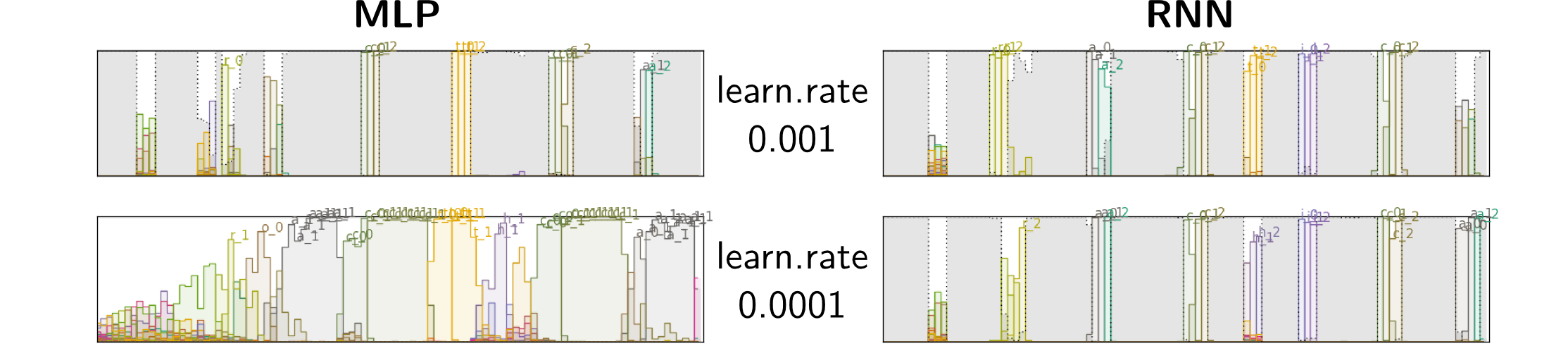
Lower learning rate To limit the impact of the high gradients on blanks at the beginning of training, and to keep more alternatives, we trained the networks with a smaller learning rate. For RNNs, peaks remained the best option, but the results were poorer. For MLP, we managed to avoid those peaks, while getting higher performances, which seems to confirm that it is too difficult or sub-optimal for an MLP to predict localized peaks.
 |
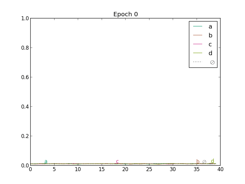
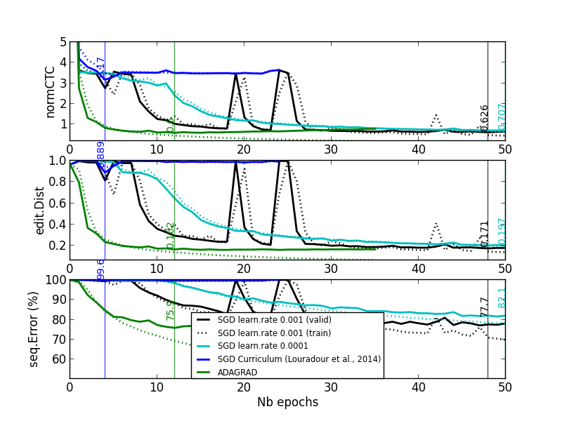
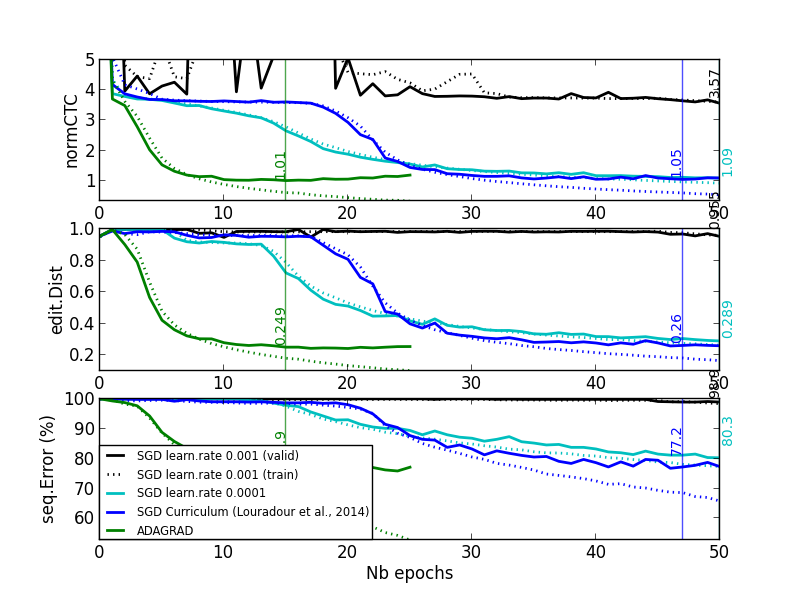
Adaptive learning rate per parameter (RMSProp) Last but not least, a similar idea to try to control the impact of the gradients for the blank label is to use an adaptive learning rate (per parameter). On more complicated databases, we sometimes observe plateaus at the beginning of CTC training. The cost value more of less corresponds to blank predictions only (see black and blue curves on the figure below). [Louradour and Kermorvant, 2014] argue that it is due to the difficulty for this training method to both align and recognize characters. They propose a training curriculum where short sequences (easier alignment task) are favoured at the beginning of training.
Following our analysis, we suppose that it is also explained by the difficulty to start predicting characters instead of blanks, because of the backpropagated error signal. Thus, we chose an training algorithm that adapts the learning rate for each parameter, according to the past gradients: RMSProp [Tieleman and Hinton, 2012]. With this approach the learning rate will be smaller if the parameter received high gradients, and bigger in the case of small gradients. From the labels perspective, we might hope that it will mitigate the high gradients coming from the blank.
In the next figure, we present the evolution of predictions under CTC training with SGD and RMSProp. This is a toy example: the values of the predictions (inputs of the CTC) are directly optimized from random initialization (there is no neural network, it only shows the dynamics of CTC training).
 |
 |
| Simple SGD | RMSProp |
On two tasks exhibiting plateauing behaviours, we see on the next plot that even if smaller learning rates or curriculum training alleviate the problem, with Adagrad (or similarly RMSProp) the problem completely vanishes:
 |
 |
| Task 1 | Task 2 |
Conclusion
We studied the CTC training algorithm, its relation to framewise and HMM training, and the role of the blank symbol in the CTC.
- CTC training is similar to:
- framewise training but sums over all possible alignments
- NN/HMM training but without transition probabilities and state priors
- It is not limited to one state per character + blank in the hybrid NN/HMM framework, but it is only interesting in that setup
- CTC+Blank works especially well with RNNs (because it asks the net to produce peaked and localized character predictions)
- It seems to give advantages for finding alignments during training and for efficient decoding
References
- [Bengio et al., 1992]
- Yoshua Bengio, Renato De Mori, Giovanni Flammia, and Ralf Kompe. Global optimization of a neural network-hidden Markov model hybrid. Neural Networks, IEEE Transactions on, 3(2):252–259, 1992.
- [Bianne et al., 2011]
- A.-L. Bianne, F. Menasri, R. Al-Hajj, C. Mokbel, C. Kermorvant, and L. Likforman-Sulem. Dynamic and Contextual Information in HMM modeling for Handwriting Recognition. IEEE Trans. on Pattern Analysis and Machine Intelligence, 33(10):2066 – 2080, 2011.
- [Bluche, 2015]
- T. Bluche. Deep Neural Network for Large Vocabulary Handwritten Text Recognition. PhD thesis, Université Paris-Sud, 2015.
- [Buse et al., 1997]
- R. Buse, Z Q Liu, and T. Caelli. A structural and relational approach to handwritten word recognition. IEEE Transactions on Systems, Man and Cybernetics, 27(5):847–61, January 1997. (doi:10.1109/3477.623237)
- [Graves et al., 2006]
- A Graves, S Fernández, F Gomez, and J Schmidhuber. Connectionist temporal classification: labelling unsegmented sequence data with recurrent neural networks. In International Conference on Machine learning, pages 369–376, 2006.
- [Haffner, 1993]
- Patrick Haffner. Connectionist speech recognition with a global MMI algorithm. In EUROSPEECH, 1993.
- [Hennebert et al., 1997]
- Jean Hennebert, Christophe Ris, Hervé Bourlard, Steve Renals, and Nelson Morgan. Estimation of global posteriors and forward-backward training of hybrid HMM/ANN systems. 1997.
- [Konig et al., 1996]
- Yochai Konig, Hervae Bourlard, and Nelson Morgan. Remap: Recursive estimation and maximization of a posteriori probabilities-application to transition-based connectionist speech recognition. Advances in Neural Information Processing Systems, pages 388–394, 1996.
- [Louradour and Kermorvant, 2014]
- Jérôme Louradour and Christopher Kermorvant. Curriculum learning for handwritten text line recognition. In International Workshop on Document Analysis Systems (DAS), 2014.
- [Senior and Robinson, 1996]
- Andrew Senior and Tony Robinson. Forward-backward retraining of recurrent neural networks. Advances in Neural Information Processing Systems, pages 743–749, 1996.
- [Tieleman and Hinton, 2012]
- Tijmen Tieleman and Geoffrey Hinton. Lecture 6.5-rmsprop: Divide the gradient by a running average of its recent magnitude. COURSERA: Neural Networks for Machine Learning, 4, 2012.
- [Yan et al., 1997]
- Yonghong Yan, Mark Fanty, and Ron Cole. Speech recognition using neural networks with forward-backward probability generated targets. In Acoustics, Speech, and Signal Processing, IEEE International Conference on, volume 4, pages 3241–3241. IEEE Computer Society, 1997.
Copyright Notice.This material is presented to ensure timely dissemination of scholarly and technical work. Copyright and all rights therein are retained by authors or by other copyright holders. All persons copying this information are expected to adhere to the terms and constraints invoked by each author's copyright. These works may not be reposted without the explicit permission of the copyright holder.